Not many people truly understand sound, but I can assure you it's one of the most impressive mathematical concepts in existence. I want to share an applied mathematical study on the manipulation of this physical phenomenon. I won't go into every physical detail behind sound, but if you can't answer this question:
What would happen if you pushed a stick stretching from Earth to the Moon?
Then you should study it, because it's a phenomenon that's present at every single moment.
Everyone knows Shazam, not the superhero, but the app that identifies a playing song in seconds. If we dig into how it works, we'll find that it uses applied sound mathematics, and on top of that, it uses the same math found in quantum physics. It's a very deep and beautiful algorithm that few people appreciate, because something so complex produces something so practical and simple.
Shazam was born in the year 2000, founded on an idea that at the time sounded almost like magic: that anyone could identify a song simply using their phone, in real time, with background noise and all. So, we're going to clone the algorithm. We're going to implement it from scratch.
There are no official papers on this algorithm, so the following implementation is an approximation of how it actually works. It's not for production use, since it's written in C from scratch. We only use libraries for real-time spectrogram visualization, to study it in depth and explain it properly. We'll talk more about that later.
Sound
Physically, sound is a wave of atoms, or more precisely, a wave of mechanical pressure. We've always heard these concepts: "waves", "pressure", "atoms", but we never dig deeper into what they actually mean.
When something vibrates (a string, a speaker, your vocal cords), it pushes the adjacent air molecules. In fact, we could say it pushes them like a spherical explosion. Those molecules compress, then expand, and that compression/expansion pattern propagates outward continuously at regular time intervals.
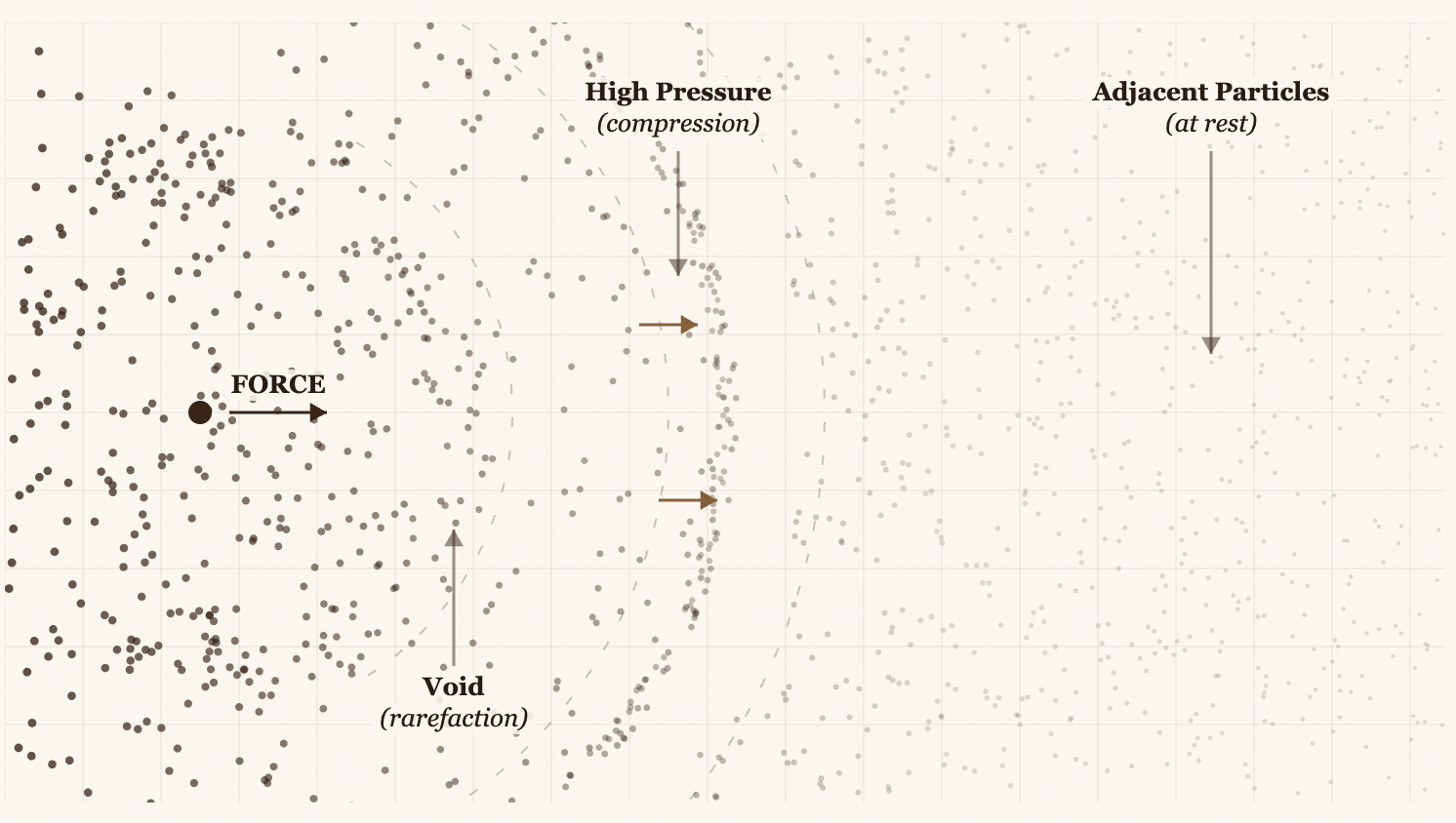
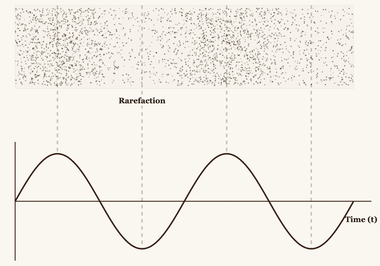
The number of times a compression/expansion cycle occurs within 1 second is the number we refer to when we say "n" Hertz. So 1 Hz tells us that one compression/expansion cycle happened exactly once during a 1-second interval. In short, it's the frequency of the waves per second. Waves are simply the compression/expansion. That's why, when you graph them, they form a trigonometric function, where compressions are the peaks of the wave and the y-axis represents the pressure of the molecules.
The high-pressure particles generate a vacuum in the surrounding space, forcing particles to rush back and fill it. But when that vacuum fills up, it pushes the particles outward again, forcing a new vacuum to form, all sustained by the original force.
The molecules that compress and expand eventually reach our ear, where their accumulation at certain intervals of the wave causes our eardrum to vibrate upon impact. Our brain then interprets the intensity of that vibration.
That is sound. And it's remarkable because it only sounds different depending on how repetitive that compression/expansion interval is. We call this frequencies, but in music, they're known as notes.
You can experiment with frequencies at the Interactive Tone Generator.
Back to the question...
Imagine a wooden stick stretching from Earth to the Moon:
If I push one end of the stick, does the other end move instantaneously?
Many would say yes, because it sounds logical, but it doesn't work that way. A stick is not rigid at a fundamental level. It's made of atoms bound together by electromagnetic forces. When you push one end, this is exactly what happens:
- You push the atoms at the Earth end
- Those atoms compress their bonds with their neighbors
- Those neighbors compress their own neighbors
- And so on...
Recognize that pattern? It's the same compression/expansion we just described. It's exactly a sound wave propagating through a solid. It's called a longitudinal compression wave, or in solid materials, an acoustic wave.
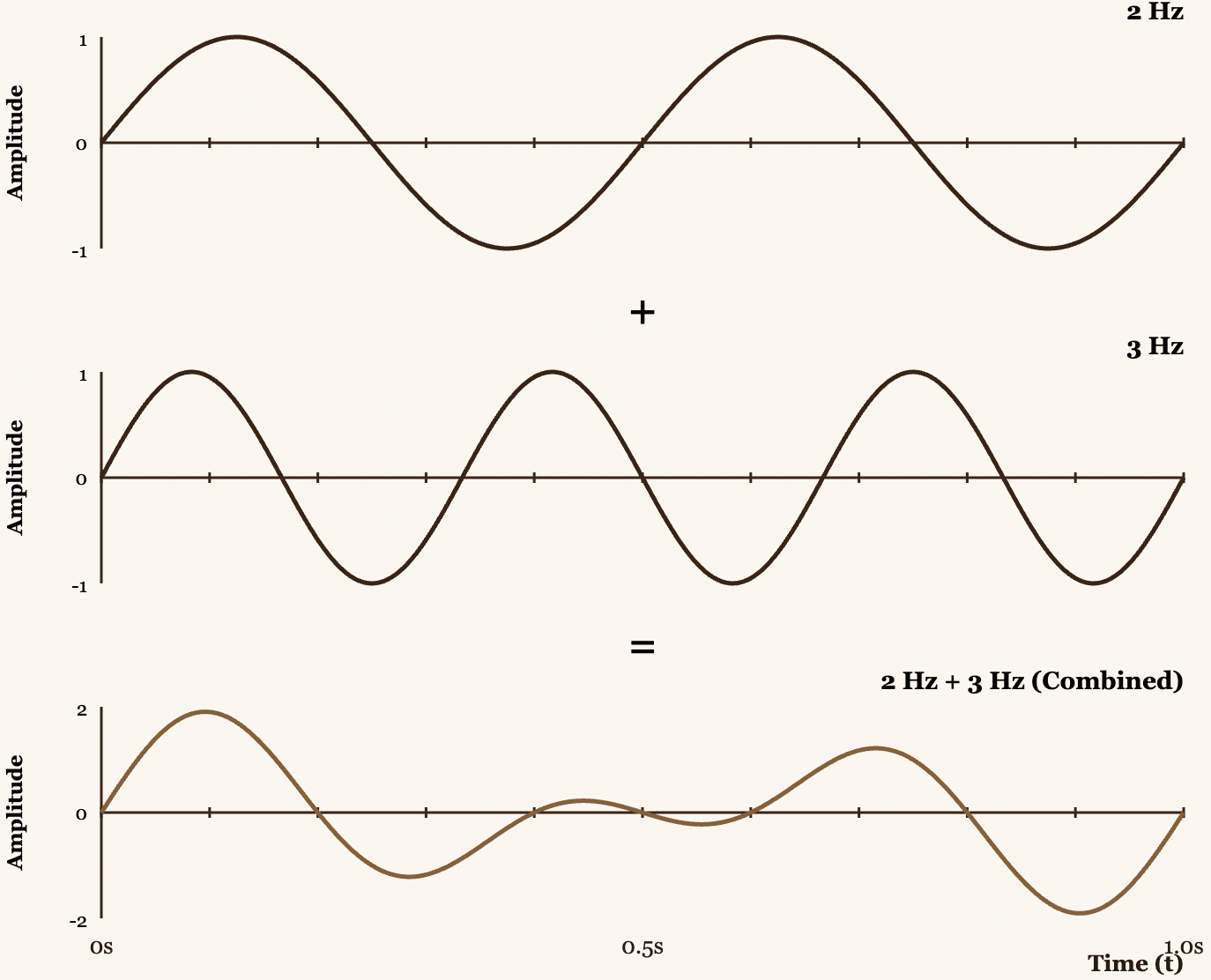
In a real environment, many compression/expansion events happen simultaneously. In music, the combination of these frequencies occurring in space produces melody. In this algorithm, we're going to separate the individual frequencies from a given mixture. This process is known as the Fourier Transform.
The "Almost" Fourier Transform
Given an audio signal , we need to build a Winding Machine to calculate the Center of Mass. But before diving into the math, let's build an intuitive understanding of what's happening.
Imagine you have an audio signal that is the sum of two pure frequencies: 440 Hz (the note A) and 294 Hz (the note D). If you graph this combined signal, you get a complex wave, the result of constructive and destructive interference between both frequencies.
Fourier's trick is to analyze the signal directly in time by "winding" it around a circle rotating at a specific frequency. This is what we call the Winding Machine.
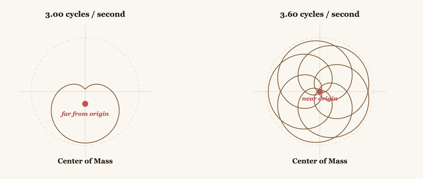
How does it work? Take your signal and wrap it around a circle rotating at, say, 3 Hz. Each point of the signal becomes a point on this rotating circle. When the signal's intensity is high, the point is farther from the origin. When it's low, it's closer.
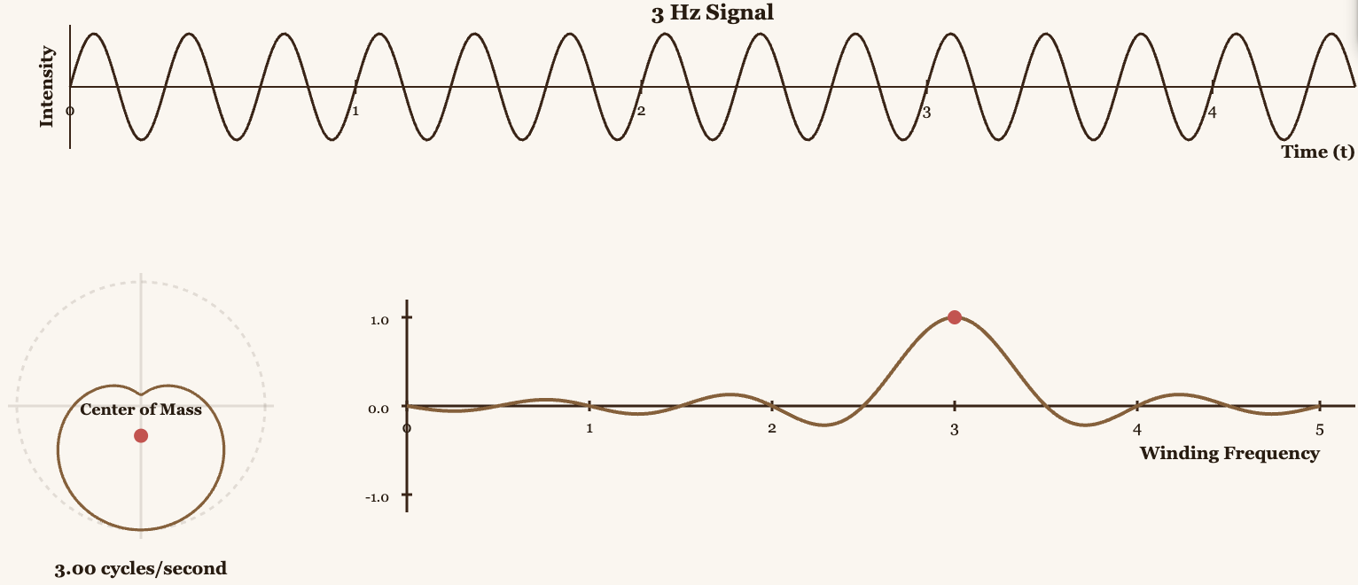
With that, we calculate the Center of Mass of all those points on the circle. This center of mass has coordinates in the plane.
If the winding frequency (3 Hz in this example) matches a frequency present in your signal, the points will consistently align in one direction, and the Center of Mass will be far from the origin. If it doesn't match, the points cancel each other out and the center of mass stays near the origin.
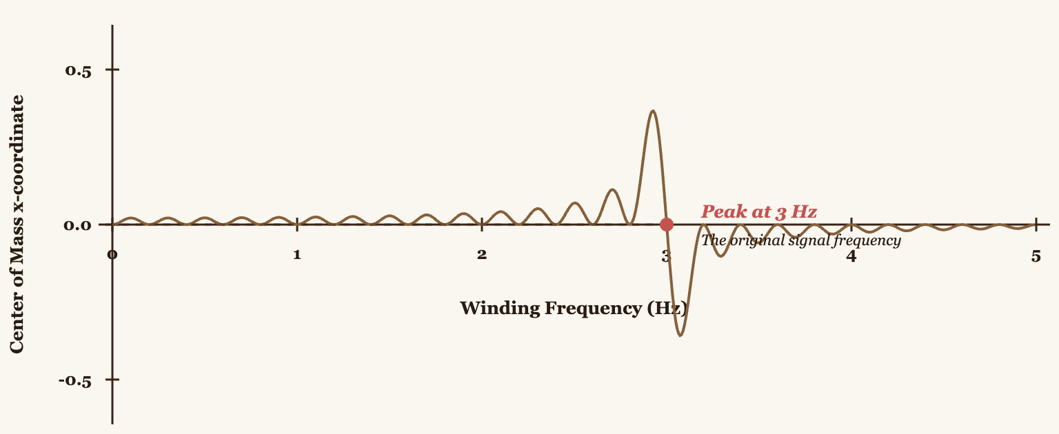
I want to be clear that what we're describing here is an "almost" Fourier Transform. Originally, only the x-coordinate of the center of mass was visualized for each winding frequency. If we plot this for all possible frequencies, we'll see peaks exactly where frequencies are present in the signal.
But here's the problem. By only using the x-coordinate, we're losing information. What about the y-coordinate? That's where complex numbers come in.
The True Fourier Transform
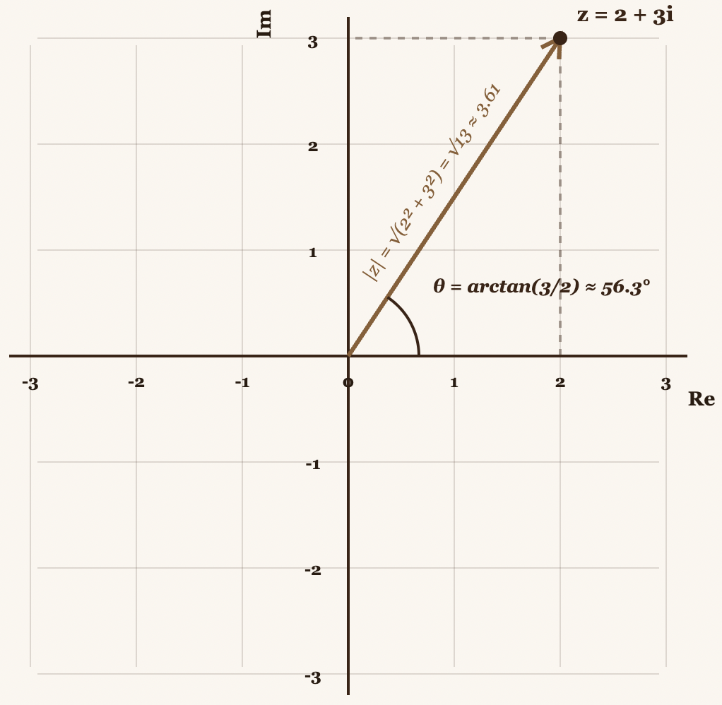
Let's think of the Center of Mass not as two separate numbers , but as a single complex number . This lets us capture all the information of the Center of Mass in a single value.
A complex number has two fundamental properties:
- Magnitude → tells you how strongly that frequency is present
- Angle (phase) → tells you at what point in the cycle that frequency begins
Both pieces of information are crucial. A 440 Hz wave that begins at a peak is different from one that begins at zero, even if both have the same frequency and amplitude.
Euler's Formula: The Perfect Winding Machine
It turns out there's a formula called Euler's formula:
This formula tells us that represents a point on the unit circle (a circle with radius 1) at angle .
Why is it perfect for winding signals? Because if we write , where is the frequency and is time, we get a point that:
- Rotates around the unit circle
- Completes exactly full revolutions per second
- Has angle at time
By convention, we use (with the negative sign) so it rotates clockwise, but this is just a mathematical convention.
Winding the Signal
Now, when we multiply our signal by , we get:
This generates the "spirograph" we observed earlier. At each instant in time :
- The angle of the point is determined by (rotating at frequency )
- The distance from the origin is determined by (the amplitude of the signal)
When is large (loud sound), the point is far away. When it's small, it's close to the origin.
The Center of Mass: The Fourier Transform
Finally, the center of mass of all those points is calculated by averaging their positions over time. This gives us a single complex number for each frequency :
Or in discrete form (for digital signals):
This complex number is the Fourier Transform of the signal at frequency .
What does it tell us?
- Its magnitude tells us how strongly that frequency is present
- Its phase tells us at what point in the cycle it begins
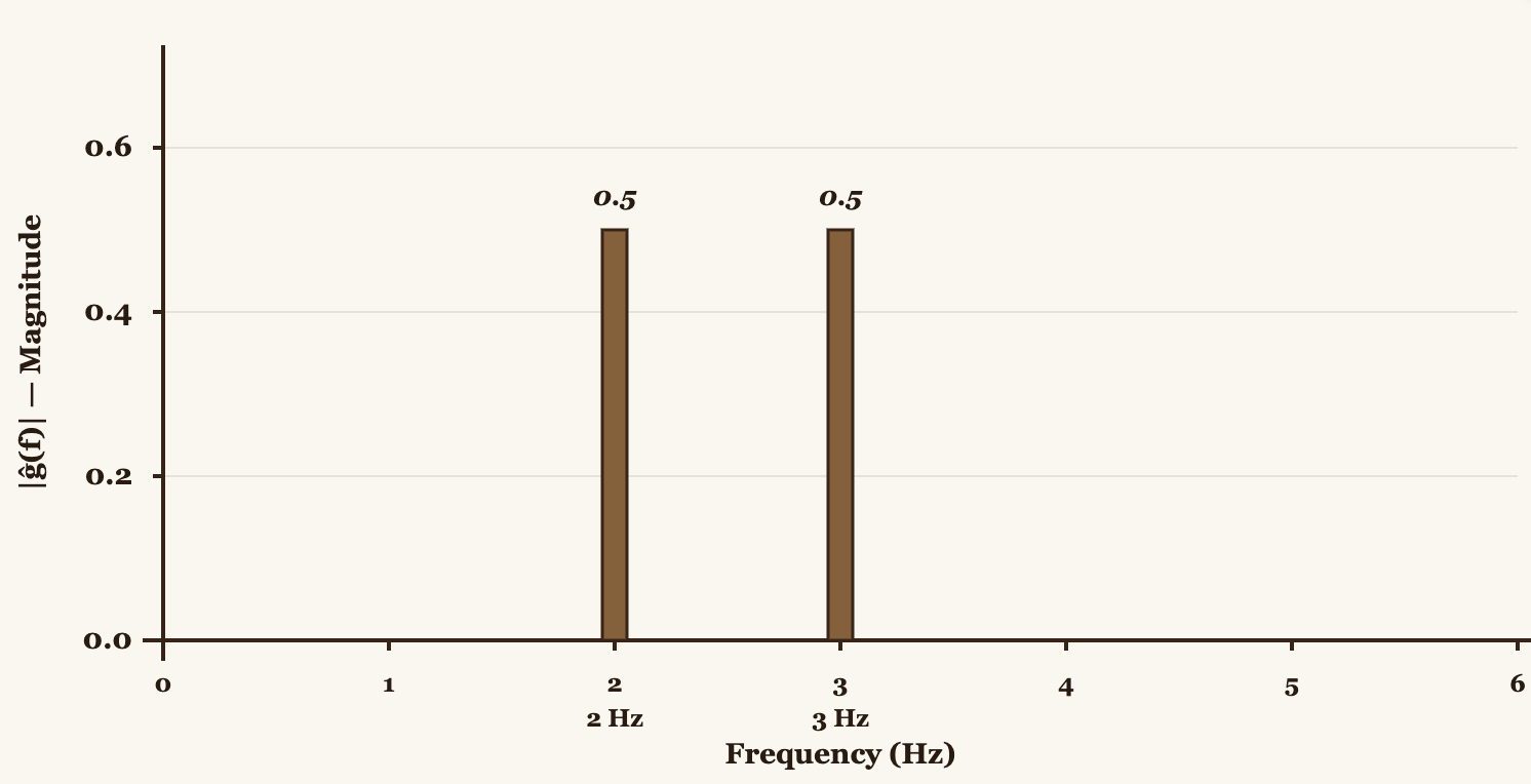
If we graph for all frequencies, we obtain the frequency spectrum of the signal, with peaks wherever frequencies are present.
This is exactly what Shazam uses as its first step: it converts audio into a spectrogram (multiple Fourier Transforms applied across time windows) to identify which frequencies are present and when. We've just separated the individual frequencies.
DFT vs FFT
In practice, when working with digital signals (like audio files), we use the Discrete Fourier Transform (DFT):
DFT: Discrete FT. is continuous; in digital audio, the domain is discrete.
And to compute it efficiently, we use the Fast Fourier Transform (FFT):
FFT: Fast Fourier Transform. It's the DFT but caching . Memoization.
FFT is simply a clever algorithm that exploits the symmetry of to avoid recomputing the same exponentials multiple times, reducing complexity from operations down to . It's what makes real-time audio processing possible.
Analog vs Digital Audio
I've used the word "digital" a lot, and that's because in practice we're only working with digital signals, but in the real world, all signals are analog.
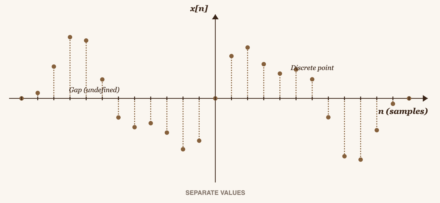
An analog signal is one that exists in spacetime and is infinitely continuous, meaning it has infinitely many points, you can't count them.
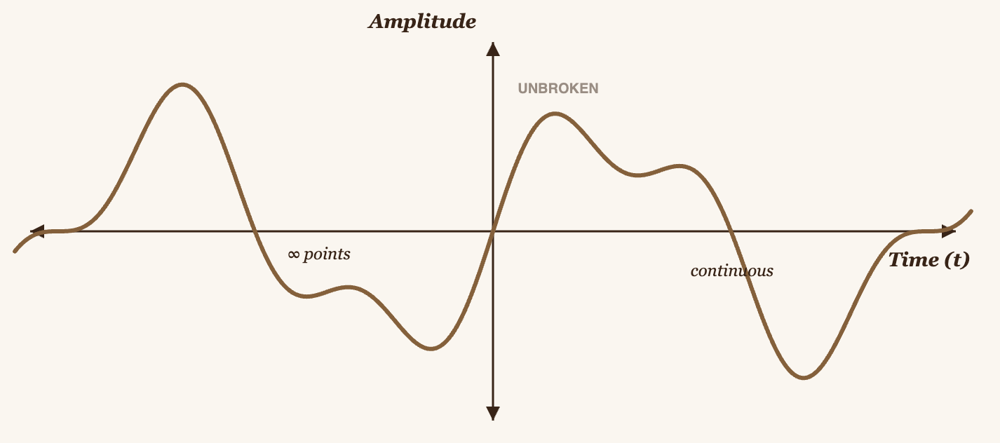
What microphones record are analog signals, but when they're stored, they become digital signals. We could call them discrete signals, because we can't store infinitely many points: we have limited computational space, not quantum. That's why we hear about audio having "resolution", the resolution is simply how many points in the signal's spacetime are stored, e.g., 44.1 kHz means 44,100 points per second. More advanced microphones can record more points, or more precisely, more frequency bins (we'll use this term shortly).
When we defined the formulas, we used integrals because in theory an integral computes the area under a curve by summing infinitely many tiny rectangles. But that expression isn't what we actually use to analyze digital signals. In practice, we use the DFT, Discrete Fourier Transform, which replaces the integral with a sum: instead of summing infinitely many points, we sum only the stored values for each time instant in our computer.
You can't integrate over a discrete space, you can only sum.
Computing DFT and STFT by Hand
We'll do this with a very small signal, because doing it by hand with a real signal (44,100 space-time points per second) would take me an eternity, but I'm a firm believer that computing things by hand (in small scenarios) is what truly makes you understand a concept.
Our Test Signal
Imagine we have a digital recording at 44,100 samples per second (44.1 kHz). Over 10 seconds, that's 441,000 samples, far too many to work with manually. So we'll simplify to understand the concept.
We'll take a time window of almost 1 second (exactly 0.9 seconds) containing only 16 samples. This will let us compute everything by hand.
Our test signal will have:
- First half (samples 0–7): a 2 Hz wave (2 cycles per second)
- Second half (samples 8–15): a 6 Hz wave (6 cycles per second)
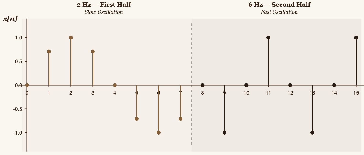
The concrete value of each sample is:
Computing the Standard DFT
The DFT formula is:
Where:
- = number of samples being analyzed (in our case, all 16)
- = frequency bin index (which frequency we're testing)
- = sample index (which sample we're analyzing)
What does "frequency bin" mean? The frequency bin is simply the frequency index. is the formula that computes the "Center of Mass" for a single frequency. To get the Center of Mass for all frequencies in the signal, we need to test every frequency, that is, compute for .
What real frequency does each represent? The frequency resolution is:
Where = sample rate = 16 Hz (16 samples per second in our simplified signal).
Therefore: Hz.
This means we're testing frequencies in steps of 1 Hz:
- → 0 Hz
- → 1 Hz
- → 2 Hz
- → 3 Hz
- ...
- → 15 Hz
Now let's compute (testing the 2 Hz frequency):
For :
Recall that , so:
Let's compute it term by term:
For :
- Angle:
For :
- Angle:
For :
- Angle:
[Continuing with all terms up to ...]
Summing all terms:
The magnitude (which is what matters for detecting frequencies) is:
This tells us there is strong energy at 2 Hz, as expected, the first half of our signal is a 2 Hz wave.
If we repeat this for all frequencies ( through ), we get:
| Frequency | ||
|---|---|---|
| 0 | 0 Hz | 0.00 |
| 1 | 1 Hz | 2.61 |
| 2 | 2 Hz | 4.00 → Strong energy |
| 3 | 3 Hz | 1.39 |
| 4 | 4 Hz | 1.41 |
| 5 | 5 Hz | 1.53 |
| 6 | 6 Hz | 4.00 → Strong energy |
| 7 | 7 Hz | 2.61 |
| 8 | 8 Hz | 0.00 |
![Bar chart showing |X̂[k]| with peaks at 2 Hz and 6 Hz](/images/the-math-of-sound-in-pure-c/dft-bar-chart.png)
We can see peaks at 2 Hz and 6 Hz. The signal had 2 Hz in the first half and 6 Hz in the second half, and DFT detected both.
The Problem with DFT: Spectral Leakage
Looking at the table: there's energy at 2 Hz and 6 Hz (as expected), but there's also "ghost" energy at other frequencies (1 Hz, 3 Hz, 4 Hz, 5 Hz, 7 Hz). This is called spectral leakage.
This happens because DFT assumes the signal is periodic and repeats infinitely. Our signal has a large discontinuity, it jumps from -0.707 (at the end of the 2 Hz wave) to 0.000 (at the start of the 6 Hz wave). This abrupt jump generates artificial frequencies.
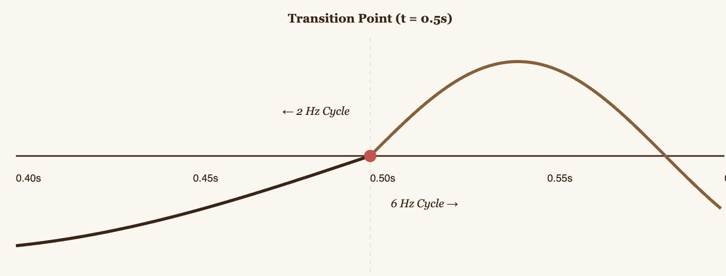
"Strong spectral leakage" means we can't precisely tell at which points in time the 2 Hz and 6 Hz frequencies are present. We only know that both are "somewhere" in the signal.
This is where the windowing technique comes in.
STFT: Short-Time Fourier Transform (DFT + Window)
The idea behind STFT (Short-Time Fourier Transform) is simple but powerful: instead of analyzing the entire signal at once, we divide it into small windows and apply DFT to each window separately.
This works because by analyzing small windows, we can capture when frequencies change over time, it's like taking "snapshots" of the signal at different moments.
The STFT formula is:
Where:
- = window index (which window we're analyzing: 0, 1, 2, ...)
- = hop size (how many samples we advance between windows)
- = window function (smooths the edges of each window)
We multiply each window by a function that equals 1 at the center and tapers smoothly to 0 at the edges. This eliminates the abrupt discontinuities that cause spectral leakage.
The Hann Window
We'll use the Hann window (also called the Hanning window):
This function creates a smooth curve that starts at 0, rises to 1 at the center, and drops back to 0.
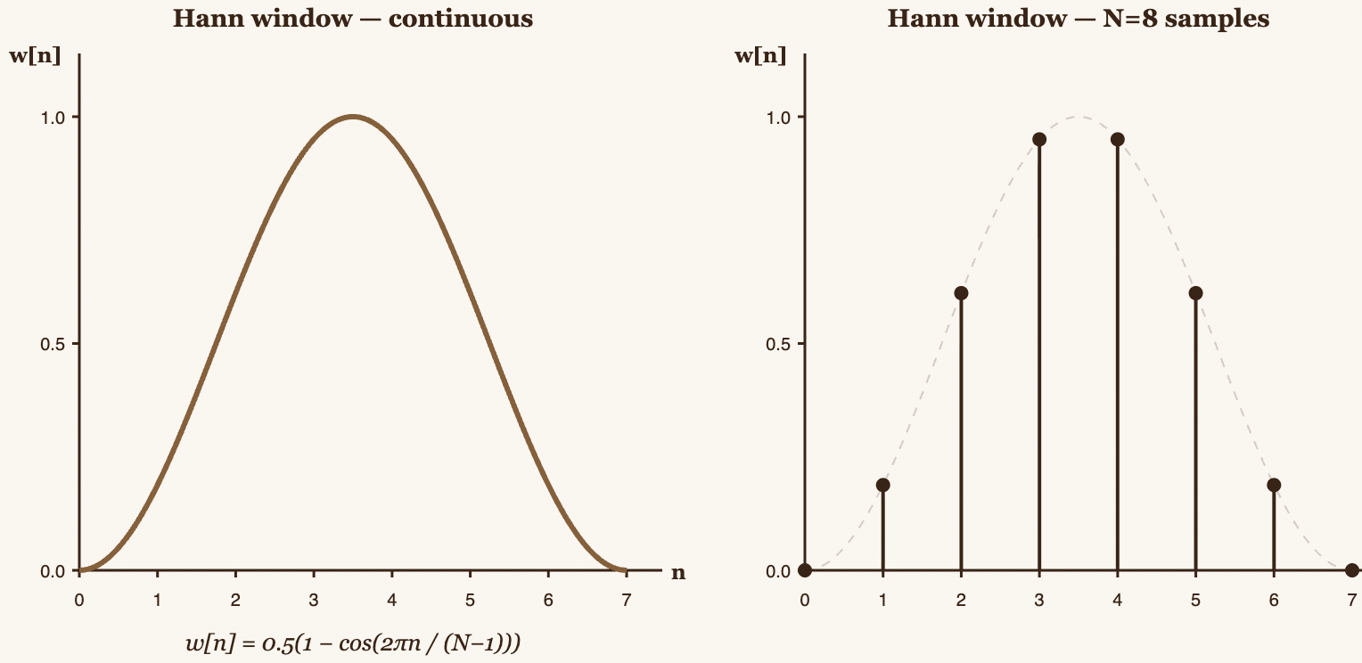
For our 16-sample signal, we'll use:
- Window size: samples (50% of the signal)
- Hop size: samples (50% overlap)
This gives us 3 windows:
- Window : samples 0–7
- Window : samples 4–11
- Window : samples 8–15
Computing STFT for Window 0
First, we compute the Hann values for :
Now we apply the window to samples 0–7 of our signal:
Windowed signal for window :
Now we compute the DFT of this windowed signal for each frequency :
| Frequency | (Window 0) | |
|---|---|---|
| 0 | 0 Hz | 0.00 |
| 1 | 1 Hz | 0.39 |
| 2 | 2 Hz | 1.06 → Strong energy |
| 3 | 3 Hz | 0.43 |
| 4 | 4 Hz | 0.00 |
| 5 | 5 Hz | 0.43 |
| 6 | 6 Hz | 0.89 |
| 7 | 7 Hz | 0.39 |
Computing STFT for Window 1
Window analyzes samples 4–11. We apply the window:
Windowed signal for window :
Results:
| Frequency | (Window 1) | |
|---|---|---|
| 0 | 0 Hz | 0.00 |
| 1 | 1 Hz | 0.43 |
| 2 | 2 Hz | 0.75 |
| 3 | 3 Hz | 0.53 |
| 4 | 4 Hz | 0.00 |
| 5 | 5 Hz | 0.53 |
| 6 | 6 Hz | 0.75 |
| 7 | 7 Hz | 0.43 |
Computing STFT for Window 2
Window analyzes samples 8–15. We apply the window:
Windowed signal for window :
Results:
| Frequency | (Window 2) | |
|---|---|---|
| 0 | 0 Hz | 0.00 |
| 1 | 1 Hz | 0.39 |
| 2 | 2 Hz | 0.49 |
| 3 | 3 Hz | 0.43 |
| 4 | 4 Hz | 0.00 |
| 5 | 5 Hz | 0.43 |
| 6 | 6 Hz | 1.06 → Strong energy |
| 7 | 7 Hz | 0.39 |
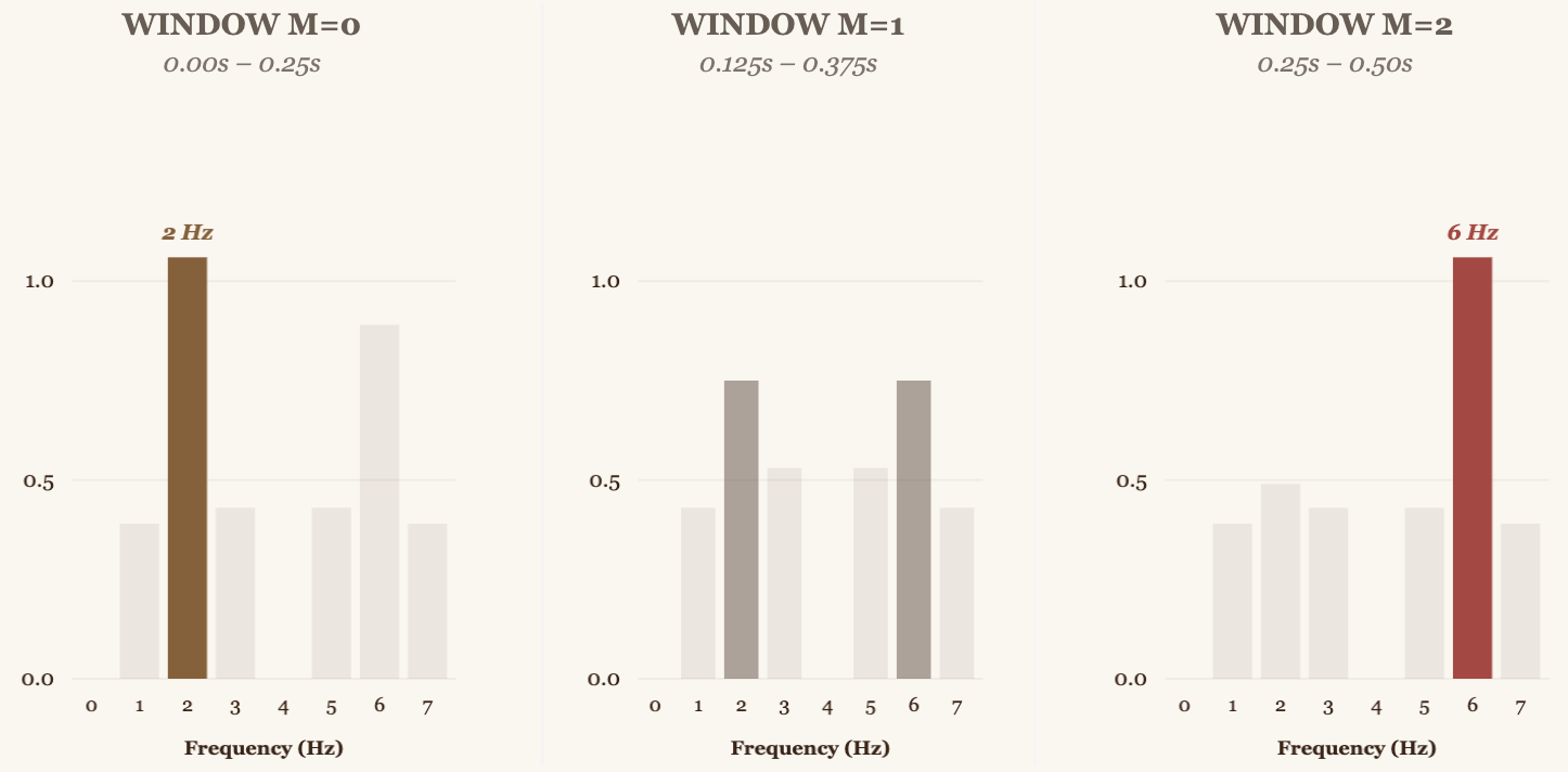
The Result: Temporal Localization of Frequencies
Now we can see exactly when the frequencies occur:
Window 0 (time 0–0.25s): Peak at 2 Hz → The signal has 2 Hz at the start
Window 1 (time 0.125–0.375s): Transition (both frequencies present)
Window 2 (time 0.25–0.50s): Peak at 6 Hz → The signal has 6 Hz at the end
This is what Shazam does: it computes the STFT of the entire song, creating a spectrogram, a 2D image where the horizontal axis is time (), the vertical axis is the frequency bin (), and the color/intensity is the magnitude .
By multiplying by Hann, we eliminate the abrupt discontinuities at the edges of each window. The values fade smoothly to zero, so DFT never "sees" artificial jumps.
That said, we should keep in mind that windowing reduces spectral leakage at the cost of some frequency resolution (peaks become wider). It's a necessary trade-off to be able to localize frequencies in time.
The Algorithm
The Fourier Transform is the core of this algorithm, without computing it first, we couldn't perform the initial analysis at all. Now we'll see how everything comes together to identify songs.
Building the Spectrogram
If we run the Fourier Transform (specifically, STFT) on a song, we'll get the frequencies present in each time window. We use a window size of 2048 samples with 75% overlap (hop size of 512 samples):
int window_size = 2048;
int hop_size = window_size / 4;  // 512 samples
int num_windows = (num_samples - window_size) / hop_size + 1;
It's a power of 2 (required for FFT), and with a sample rate of 44.1 kHz, it gives us a temporal resolution of ~46ms per window and a frequency resolution of ~21.5 Hz. A good balance between temporal and frequency precision.
For each window, we apply the Hann window (pre-computed at startup for efficiency):
float *pre_computed_windows = (float *)malloc(window_size * sizeof(float));
for (int i = 0; i < window_size; i++) {
    pre_computed_windows[i] = hann(i, window_size);
}
Where the hann() function is:
float hann(int n, int N) {
    return 0.5 * (1.0 - cos(2.0 * M_PI * n / (N - 1)));
}
Then, for each window, we multiply the samples by the window and apply FFT using the Cooley-Tukey radix-2 algorithm:
for (int m = 0; m < num_windows; m++) {
    int start_sample = m * hop_size;

    // Apply the window to the samples
    for (int n = 0; n < window_size; n++) {
        stft[m][n] = samples[start_sample + n] * pre_computed_windows[n];
    }

    // FFT in-place
    fast_fourier_transform(stft[m], window_size);
}
We use the iterative method with bit-reversal permutation. It's , much faster than the naive DFT at .
The result is a matrix stft[num_windows][window_size] where each cell contains a complex number. The magnitude tells us how strongly frequency is present in time window .
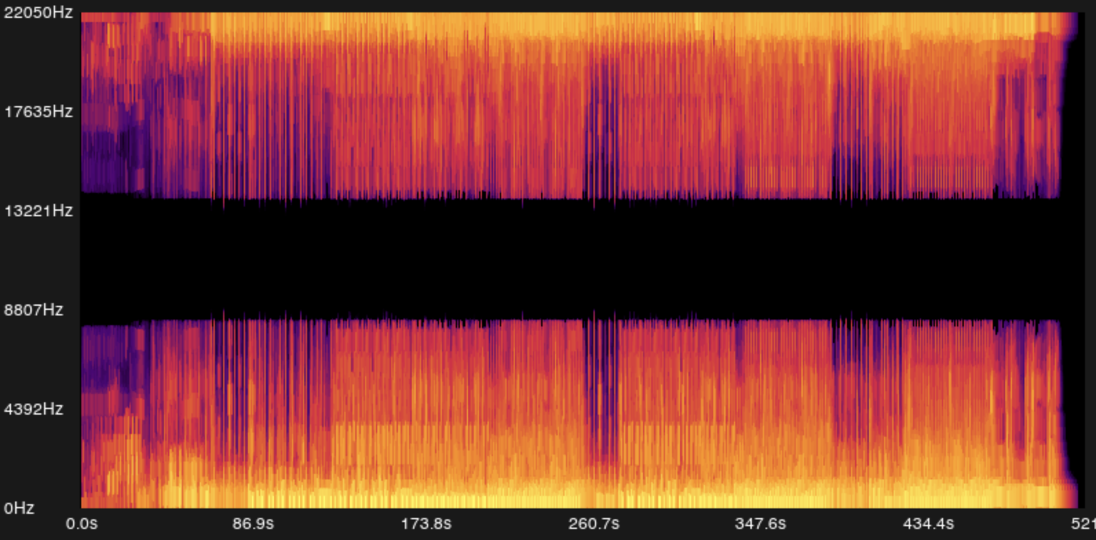
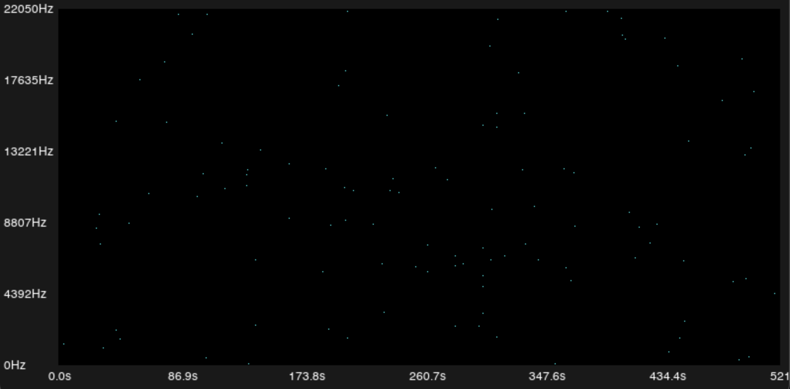
This creates our spectrogram, a 2D image of time (horizontal) vs frequency (vertical), where color intensity represents the energy at each frequency bin at each moment.
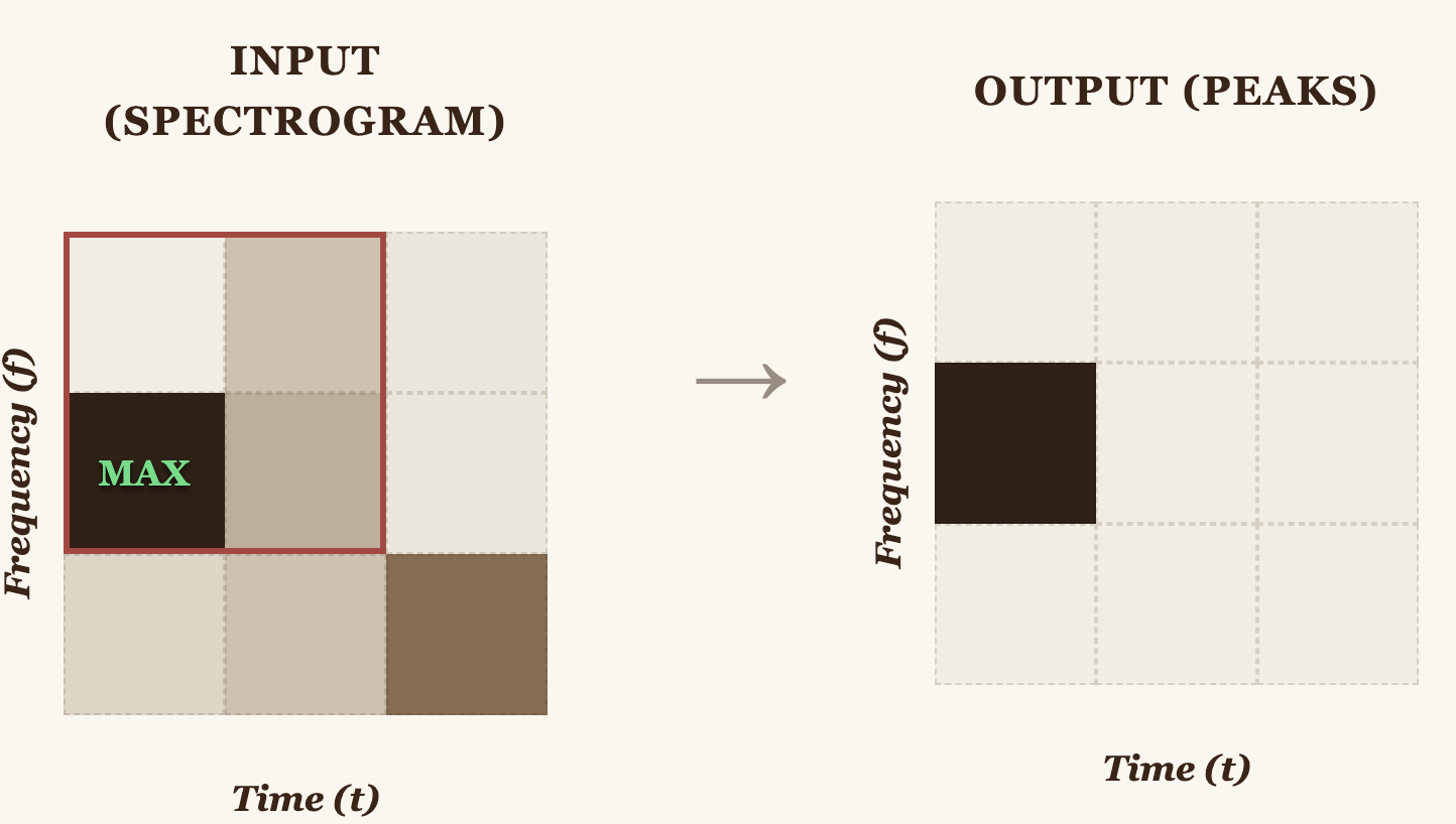
Peak Detection: Finding the Constellation Map
We can't use all the frequencies from a song as a fingerprint to compare against others, there would be too much data, and too much noise. So we use only the most prominent peaks from the spectrogram.
How do we identify peaks? With a 2D max filter. The idea: a point is a peak if it's the local maximum within its neighborhood.
Two 1D passes instead of one 2D pass, reducing complexity from to :
const int max_filter_radius = 20;

// Pass 1: Horizontal (time axis)
for (int m = 0; m < num_windows; m++) {
    for (int k = 0; k < half_window; k++) {
        float max_val = 0.0f;
        for (int dm = -max_filter_radius; dm <= max_filter_radius; dm++) {
            int mm = m + dm;
            if (mm >= 0 && mm < num_windows && mag[mm][k] > max_val)
                max_val = mag[mm][k];
        }
        temp[m][k] = max_val;
    }
}

// Pass 2: Vertical (frequency axis)
for (int m = 0; m < num_windows; m++) {
    for (int k = 0; k < half_window; k++) {
        float max_val = 0.0f;
        for (int dk = -max_filter_radius; dk <= max_filter_radius; dk++) {
            int kk = k + dk;
            if (kk >= 0 && kk < half_window && temp[m][kk] > max_val)
                max_val = temp[m][kk];
        }
        max_filtered[m][k] = max_val;
    }
}
Then we compare the original spectrogram against the filtered one. If a point has the same value in both, it is a local maximum, a peak:
for (int m = 0; m < num_windows; m++) {
    for (int k = 0; k < half_window; k++) {
        float orig = magnitude(stft[m][k]);
        if (orig == max_filtered[m][k] && orig > 0.0f) {
            is_peak[m][k] = 1;
            num_peaks++;
        }
    }
}
In a typical 3–4 minute song, this reduces millions of spectrogram points down to just ~10,000–50,000 peaks. These peaks form what Wang and Ogle call the constellation map.
Fingerprint: Hashing Peak Pairs
A single peak isn't distinctive enough. There might be a peak at 440 Hz at second 2.5 in thousands of songs. But the combination of two peaks with specific frequencies and a specific temporal gap between them is far more unique.
The strategy is:
- Take each peak as an anchor
- Define a target zone ahead in time
- Pair the anchor with up to 10 peaks in that zone
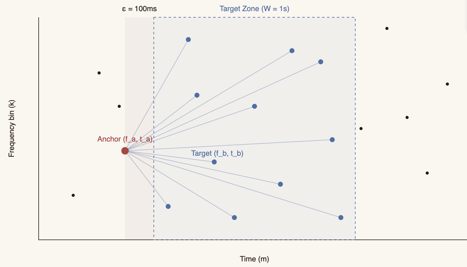
float epsilon = 0.1f;  // 100ms dead zone ahead
float W = 1.0f;         // 1 second target zone width

int epsilon_frames = (int)(epsilon * header.sample_rate / hop_size);
int W_frames = (int)(W * header.sample_rate / hop_size);

for (int m = 0; m < num_windows; m++) {
    for (int k = 0; k < half_window; k++) {
        if (is_peak[m][k]) {
            int target_zone_m_start = m + epsilon_frames;
            int target_zone_m_end = m + W_frames;

            int fan_out_count = 0;
            for (int m_target = target_zone_m_start;
                 m_target <= target_zone_m_end && fan_out_count < MAX_FANOUT;
                 m_target++) {
                for (int k_target = 0;
                     k_target < half_window && fan_out_count < MAX_FANOUT;
                     k_target++) {
                    if (is_peak[m_target][k_target]) {
                        // Create hash for this pair
                        uint64_t f_a = (uint64_t)(k * 1024 / half_window);
                        uint64_t f_b = (uint64_t)(k_target * 1024 / half_window);
                        uint64_t delta_t = (uint64_t)(m_target - m);

                        uint64_t hash = (f_a << 20) | (f_b << 10) | delta_t;

                        hashes[hash_count].hash = hash;
                        hashes[hash_count].song_id = song_id;
                        hashes[hash_count].t_anchor = m;
                        hash_count++;

                        fan_out_count++;
                    }
                }
            }
        }
    }
}
The 30-bit hash is built like this:
- 10 bits for the anchor frequency (): range 0–1023 (~20 Hz resolution)
- 10 bits for the target frequency (): range 0–1023
- 10 bits for the time difference (): range 0–1023 windows (~0 to 11.6 seconds)
This gives us billion possible combinations. More than enough to distinguish songs.
Crucially, we store the anchor time () separately, not inside the hash. This is what enables time-invariant matching: the hash is identical regardless of where in the song it appears, but lets us reconstruct the temporal offset.
A 3-minute song generates approximately 50,000–200,000 hashes. These are stored as:
{
  "hashes": [
    {"hash": 1234567890, "song_id": 0, "t_anchor": 42},
    {"hash": 9876543210, "song_id": 0, "t_anchor": 43},
    ...
  ]
}
Matching: The Temporal Offset Histogram
To identify a song, we follow the same process:
- Record an audio sample (e.g., 5–10 seconds)
- Generate its spectrogram
- Detect peaks
- Create hashes the same way
Now we have two sets of hashes:
- Query hashes: from the sample we want to identify
- Reference hashes: from all songs in the database
Matching is done with a Python script (matches.py):
# Load reference hashes
ref_hashes_dict = {}
for hash_file in args.hash_files:
    with open(hash_file) as f:
        data = json.load(f)
    for h in data["hashes"]:
        ref_hashes_dict[h["hash"]] = h

# Find matches
matches = [h for h in query["hashes"] if h["hash"] in ref_hashes_dict]
But simply counting how many hashes match isn't enough. We need to verify that they match consistently over time.
For each matching hash, we compute the delta_t (time difference):
match_data = []
for match in matches:
    ref_entry = ref_hashes_dict[match["hash"]]
    delta_t = ref_entry["t_anchor"] - match["t_anchor"]
    song_id = ref_entry["song_id"]
    match_data.append((song_id, delta_t))
If the sample truly comes from the reference song, all matching hashes should have approximately the same delta_t, because they originate from the same segment of time.
We visualize this with a histogram:
for ax, sid in zip(axes, song_ids):
    dts = [dt for s, dt in match_data if s == sid]
    ax.hist(dts, bins=50, edgecolor="black", alpha=0.8)
    ax.set_title(f"Song ID: {sid}")
    ax.set_xlabel("delta_t (ref t_anchor - query t_anchor)")
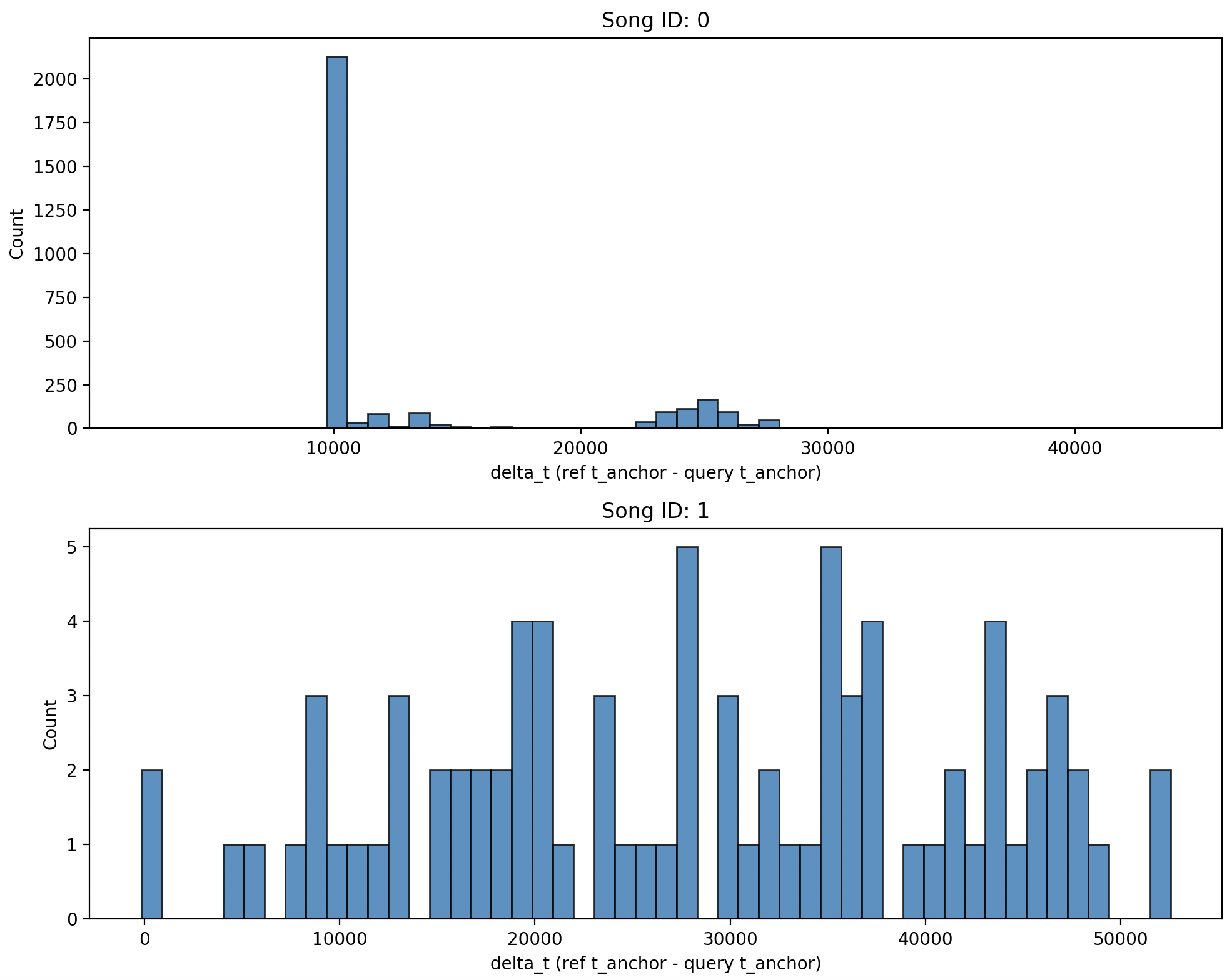
If there's a match, we'll see a large, narrow peak in the histogram. That peak tells us:
- The song (song_id)
- Where in the song the sample comes from (the delta_t value at the peak)
If there's no match, the delta_t values will be scattered randomly, with no clear peaks.
The complete code is available at: Shazam Algorithm. It's not for production, but it's perfect for understanding how Shazam works internally. Every line of code was written with the goal of understanding, not just making it work.
pfff :)