Building an LLM From Scratch · Bernardo's Blog

There is no such thing as Artificial Intelligence. It's nothing more than an enormous mathematical function. What they call AI is a function $f$ that takes numbers and returns numbers. What changes between what runs on my laptop and what runs in a datacenter is the size of that function. Below, I'm going to explain how a Large Language Model (LLM) works, building one from scratch, no libraries, no PyTorch, no NumPy, no autograd, no GPU. All of it running on a MacBook Air M2 with 8 GB of RAM.

The same thing is going to happen that happened with computers. We have all used or own a computer, and I'm 100% sure almost nobody can explain how one works. This leads us into ignorance when we make decisions or when we listen to other people talk about a topic they don't even understand. I talk more about that here. That's why I set myself the goal of doing this project, so I could explain how it works and show visually how these artificial neurons behave. In the end we're going to see that it's a pretty dumb machine, but that something dumb, if you stack it enough times, becomes something very complex. From the two states a bit has (0 and 1) we got to a computer.

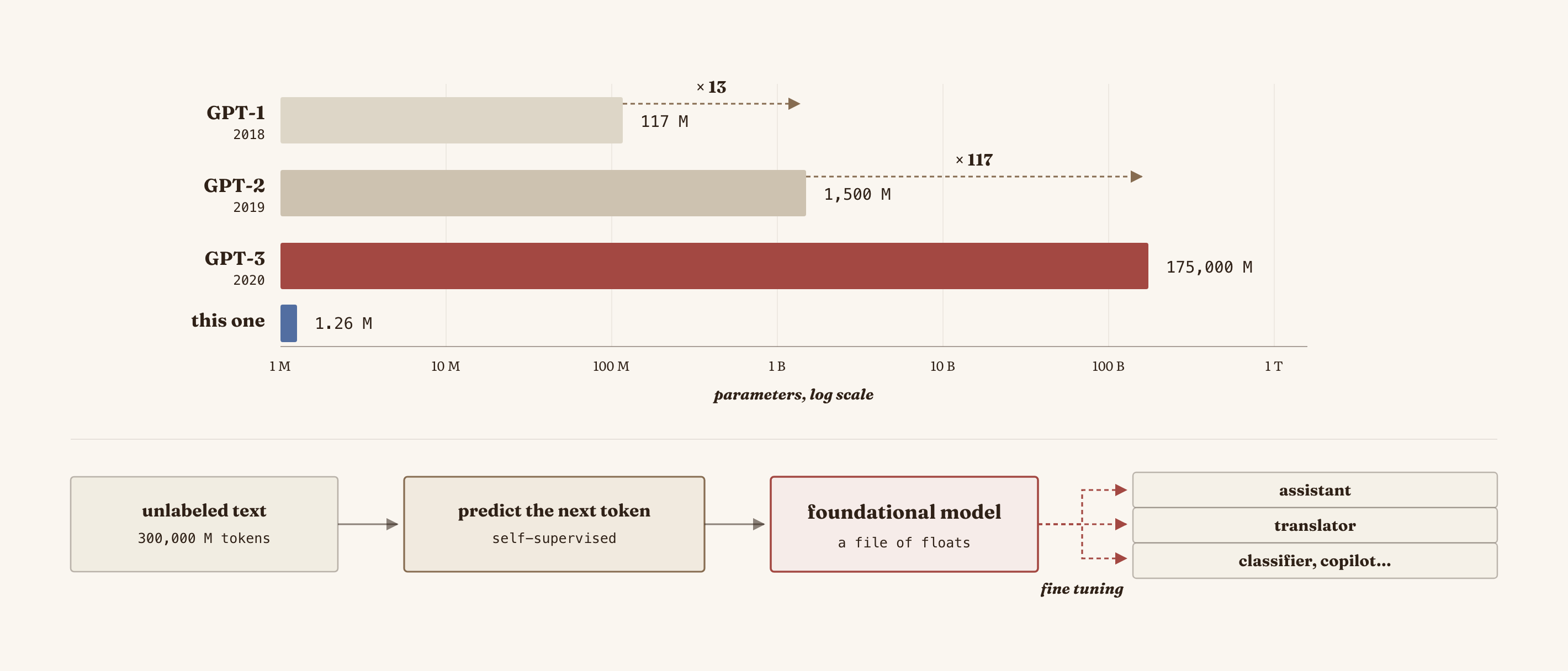
An LLM is only a function with billions of parameters. The model we're going to build has 1,258,240 parameters, which is very little compared to GPT-3 (the model that gave rise to ChatGPT, with 175 billion). We're going to see that 1.26 million parameters isn't enough, but honestly it's still very dumb. It's as if the human brain had only 1.26 million neurons, it couldn't do anything.

We know GPT-3's parameter count because OpenAI published it in 2020. The ones for GPT-3.5, GPT-4 and onward were never published. It's a trade secret.

Where did it come from?

It's worth telling the story because almost everything people believe was invented in 2022 is between 30 and 300 years old. Also, the term AI (Artificial Intelligence) isn't the right one, we just say it that way so people understand what it's about, but these are really Deep Learning models.

They are three different things:

Artificial Intelligence is any machine that imitates something a human does. A chess engine full of rules written by hand by a person is also AI. Nothing learns there, it's pure if.
Machine Learning is a subset. Instead of you writing the rules, you give the machine examples and it finds the rules on its own. You still decide which features to look at, what we call "labels" (the size, the color, the price).
Deep Learning is a subset of the previous one. You use neural networks with many layers, and now you don't even decide which features matter. The machine discovers that on its own too.

Recurrent Neural Networks (RNN)

Before 2017, to process text, Recurrent Neural Networks (RNN) were what people used. Basically, this is how they work... If language is a sequence, let's process it as a sequence. The network reads word 1, saves a summary of what it has so far (hidden state), reads word 2, updates the summary, and so on.

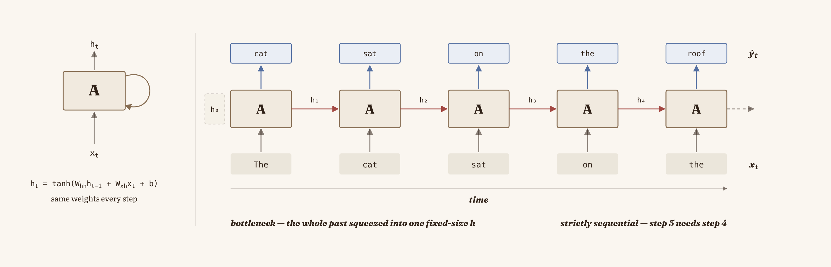
Diagram of how an RNN works — An RNN reads one at a time and has to summarize the whole past into a single vector.

This had two problems.

The first is that the entire past has to fit into a single vector. If you translate a 40 word sentence, by the time the network reaches the end, what it read at the beginning is already lost. It's a bottleneck.

The second is that an RNN can't be parallelized. To compute step 5 you need the result of step 4. It doesn't matter if you have ten thousand GPUs, it's sequential. Number two can't start until number one finishes. You're forced to go one at a time.

Attention Is All You Need

In 2017, a team at Google published a paper called "Attention Is All You Need". A proposal to solve the problem the RNN model had... short term memory, because when a string of text was long, it no longer made sense. In short, it couldn't pay attention to the beginning of the text.

In a way, attention was already being used in RNNs as a patch to improve how they worked. What this paper did was remove everything else. They threw out recurrence completely and kept only this patch. And it turned out the patch was the engine. They called that model the "Transformer".

The transformer didn't win by being mathematically deeper. It won because it parallelizes.

In attention, all positions are compared against all positions at the same time, in a single matrix multiplication. There's no dependency between steps. And a GPU is, essentially, a matrix multiplying machine.

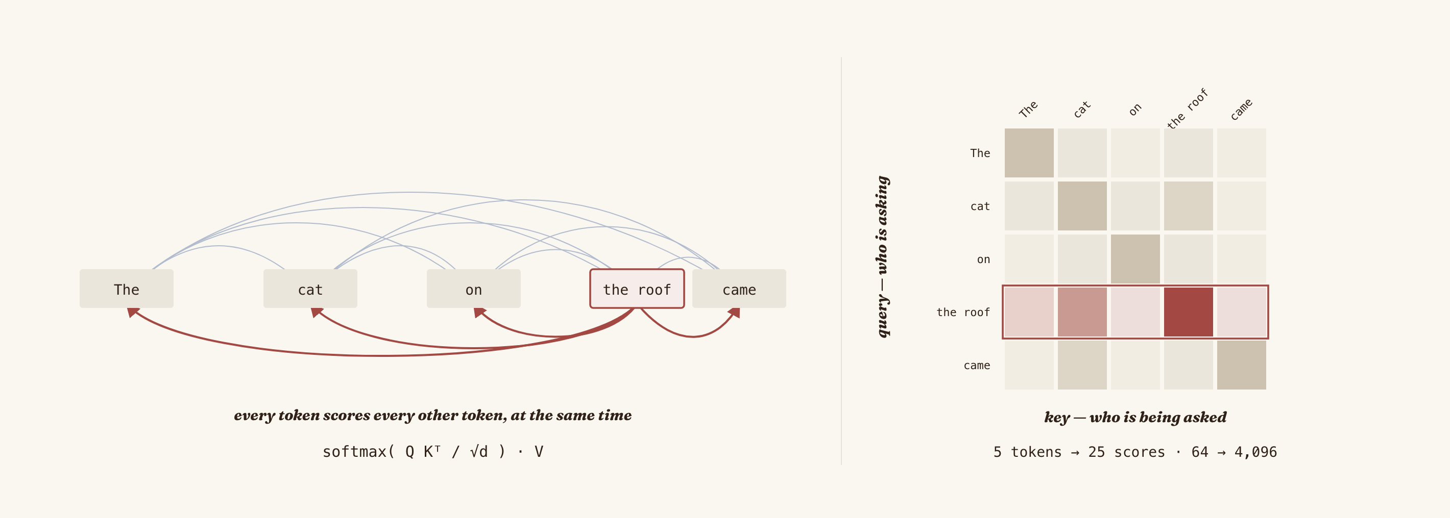
The attention mechanism: each position is compared against all the others — Attention compares all positions at the same time, in a single matrix multiplication.

So the transformer is an architecture that fit perfectly into the hardware that already existed. I know the concept of attention sounds strange and is hard to visualize, but below I'm going to show how all of it looks.

GPT and BERT

The original transformer came with two parts, because it was designed to translate. An encoder that read the sentence in one language, and a decoder that wrote it in the other.

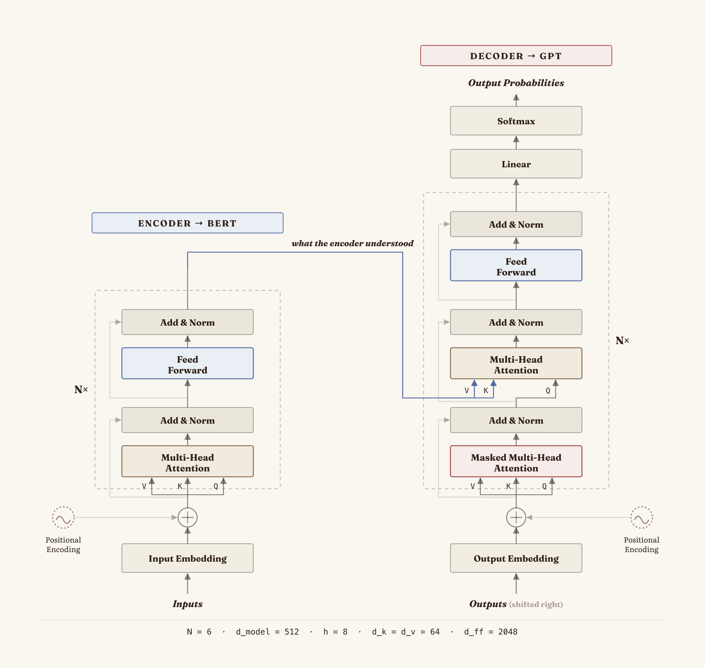
The original transformer architecture: encoder and decoder — The 2017 transformer. Google kept the encoder, OpenAI the decoder.

The interesting part is that the two biggest companies each grabbed one half.

Google kept the encoder and in 2018 released BERT (Bidirectional Encoder Representations from Transformers). The encoder can see the whole sentence, forward and backward at the same time, and that's why BERT is very good at understanding text, classifying, searching, analyzing sentiment. In fact Google put it into its search engine in 2019. What BERT can't do is write, because to write you can't see the future.

OpenAI kept the decoder and released GPT, which stands for Generative Pre-trained Transformer:

Generative, because it generates. It predicts the next token, one by one. We're going to explain that further down.
Pre-trained, because first it's trained on a mountain of unlabeled text (the task is simply to guess the next word, which is free, you don't need a human to label anything) and afterwards it's tuned for specific tasks. This is known as a Foundational Model, and the tuning for specific tasks is what we call fine tuning.
Transformer, for the 2017 architecture.

So GPT and BERT are simply Foundational Models, which were later fine tuned to specialize in something useful, like an assistant, a translator, among other things.

The decoder can only look backward. That restriction is called a causal mask and we're going to program it when we build the attention module. It is, literally, putting $-\infty$ in the upper half of a matrix. All the ability to write comes out of that.

During 2018 and 2019 the model everyone loved was BERT. GPT-1 had 117 million parameters and impressed nobody. What OpenAI did differently wasn't a new idea, it was not changing the architecture and only making it bigger, 117 million in 2018, 1.5 billion in 2019, 175 billion in 2020.

Growth of GPT parameters from GPT-1 to GPT-3 and the concept of a foundational model — From GPT-1 to GPT-3: the same architecture, 1,496 times more parameters.

How an LLM uses text

A model doesn't read. It doesn't know what a letter is, or a word, or a language. The only thing it knows how to do is multiply numbers and add them. Very close to what a computer knows too. So the first problem, before attention and before anything that sounds "intelligent", is how to turn text into numbers, and those numbers into geometry. Why? To give them meaning, a distance, something we can measure.

But first... what is a tensor?

In PyTorch we use it as torch.tensor(...) and that's it. In C there's nothing, so you have to write it. Since we're doing this from scratch, we also have to write our own tensor library.

A tensor sounds like something elegant, multidimensional, abstract. But it's simpler... It's only a 1 dimensional vector in memory (that is, in RAM) with metadata

typedef struct {
    float *data;    // flat array
    int *shape;     // e.g {2, 4, 768}
    int *strides;   // precomputed strides
    int ndim;       // number of dimensions e.g 3
    int size;       // total elements = 2*4*768 = 6144
    float *grad;
} Tensor;

A 3 dimensional tensor doesn't exist. There are no cubes in memory. RAM is vertical, according to the Von Neumann architecture, a single line of bytes, and it always has been. The only thing there is is a flat array of 6,144 floats and four integers that tell us how to build it, "2×4×768".

Dimensions in computing are an abstraction.

What makes the abstract possible are the strides. If I want the element at position $(i, j, k)$ of a tensor with shape $[B, T, C]$ , the real address in the strip is:

\text{flat index} = i \cdot (T \cdot C) + j \cdot C + k

A stride is how many floats you have to jump to advance one step along that axis. To advance one position on the last axis, you jump 1. To advance one on the middle axis, you jump $C$ . To advance one on the first, you jump $T \cdot C$ . I precompute them once when creating the tensor so I don't recompute multiplications on every access:

int *strides = (int *)malloc(ndim * sizeof(int));
strides[ndim - 1] = 1;
for (int i = ndim - 2; i >= 0; i--) {
    strides[i] = strides[i + 1] * shape[i + 1];
}

Changing the shape of a tensor is easy. Not a single byte moves. You just rewrite four integers and that's it, the same data now has a different shape. A tensor of $[2, 4, 768]$ becomes one of $[8, 768]$ without copying anything, because in memory they were always the same 6,144 floats in the same order.

Now, being honest, the following functions of the library: tensor_matmul, tensor_transpose and tensor_reshape I made with AI's help, and I left it written in the code:

// damn... matmul, transpose, and tensor_reshape needed days studying the perfect shape,
// but honestly, they were not the point of this practice, so, yes, another one made with AI.

:) The point of this project wasn't to prove I can write a triple loop with indices, it was to understand the mechanism of the model.

Text has to become numbers

The model only understands numbers and we write letters. Somebody has to assign a number to each piece of text. The question is to which pieces.

There are three ways to do it.

Option 1: one number per letter. a is 1, b is 2, and so on. With about a hundred numbers we cover everything. But doing it this way has two problems. The problem with this is that we're asking the model to reconstruct the entire language from scratch, letter by letter. It's not going to work.

Option 2: one number per word. "house" is 4,102. Each number already has meaning. But even so, it's not the ideal way:

The catalog explodes. Spanish conjugates everything: cantar, canto, cantas, cantaba, cantaría, cantaríamos... Each one would need its own number, and none would share anything with the others even though they're the same word. Add plurals, diminutives and proper names, and you're already in the hundreds of thousands.
And sooner or later a word arrives that isn't in the catalog. A name, a typo, a word in another language, a term that got invented because we wrote the prompt wrong. The model goes blind right there.

Option 3: one number per piece of a word. If "cantaba" is split into cant + aba, then "cantar" can reuse the piece cant. With a few thousand pieces you can assemble any word, including the ones you never saw. In the worst case you assemble them letter by letter.

Each one of those pieces is what we call a token. And the complete catalog of pieces the model knows is what we call the vocabulary.

It's worth understanding how literal this is. When I say my model has a vocab_size of 2,048, I mean that exactly 2,048 pieces of text exist in its entire universe, numbered from 0 to 2,047. There is no 2,048. Any text you give it, in any language, has to be expressed by combining those 2,048 pieces. GPT-2 has 50,257. It's a closed vocabulary, and it's defined before the model exists.

But, who decides which pieces they are?

In this case, the one deciding isn't a human, or a professional, it's decided by frequency.

The tokenizer

The method GPT-2, GPT-3, GPT-4 and Llama use to do exactly what we explained above, splitting words into pieces by frequency, is called Byte Pair Encoding (BPE). It's funny because BPE was published by Philip Gage in 1994, in the C Users Journal, and it was a data compression algorithm. Its purpose was to make files smaller. It had nothing to do with language, or with neural networks. In 2016 someone realized it was useful for splitting words, and ever since, we use it.

C Users Journal was a magazine for C programmers.

The Byte Pair Encoding (BPE) algorithm

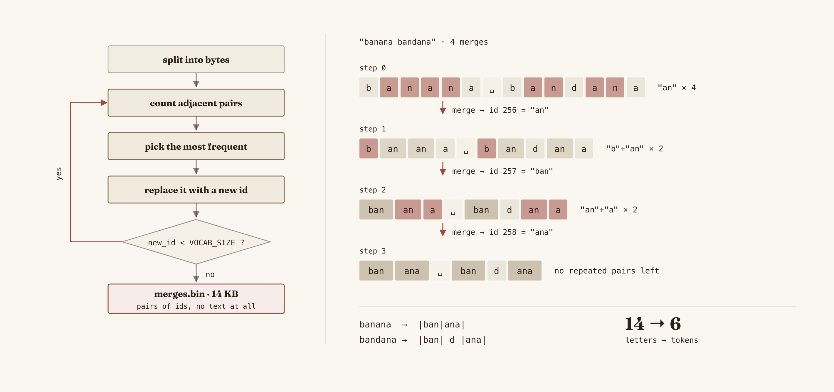
Flow diagram of the BPE algorithm: count pairs, pick the most frequent, replace, repeat — Count pairs, pick the most frequent one, replace it, repeat.

We start with the text split into the smallest possible units. One per letter.
We count the neighbor pairs that appear the most times.
That pair becomes a new piece. We give it a number and replace all of its occurrences.
We repeat until we reach the vocabulary size you wanted.

Each repetition is called a merge, and the ordered list of merges is the tokenizer.

The best thing is to see it running. If we give it the text "banana bandana", and ask for 4 merges:

#### "banana bandana"  (4 merges)
  step 0: |b|a|n|a|n|a| |b|a|n|d|a|n|a|
  merge -> id 256 = "an" (appeared 4 times)
  step 1: |b|an|an|a| |b|an|d|an|a|
  merge -> id 257 = "ban" (appeared 2 times)
  step 2: |ban|an|a| |ban|d|an|a|
  merge -> id 258 = "ana" (appeared 2 times)
  step 3: |ban|ana| |ban|d|ana|
  (no repeated pairs left)
  14 letters -> 6 tokens

At step 0 nothing has been learned, each letter is its own token. The pair that appears the most is an, four times, so an becomes token 256 and the text is rewritten using it. Now ban appears twice, it becomes 257. Then ana, 258. And it stops on its own right there, because there are no repeated pairs left.

It sounds strange that we start at 256, but it makes sense because the possible combination of bytes is 256 (ASCII table). I'll explain it below.

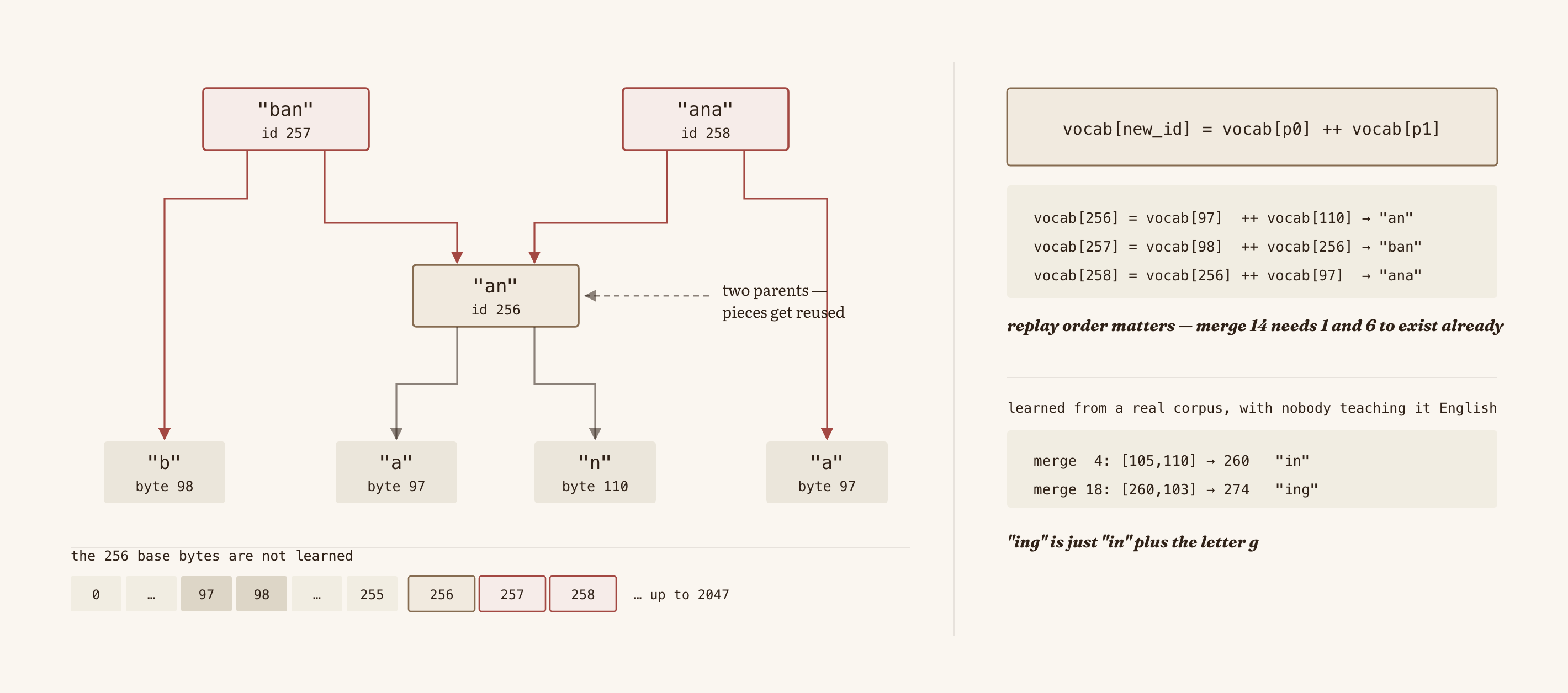
We can see that token 257 (ban) is made of the letter b plus token 256 (an). Pieces are built on top of previous pieces. The vocabulary is like a tree... each new token leans on the ones that already existed, and if you keep going down you always end up at letters.

Merge tree: token 257 leans on 256, and going down you always reach letters — Each new token leans on the previous ones, and at the bottom there are always bytes.

In the end, we get this:

banana   ->  |ban|ana|
bandana  ->  |ban| d |ana|

The two words ended up sharing pieces. The model doesn't see them as two unrelated things, it sees them assembled from the same pieces plus one difference. Also, 14 letters became 6 tokens. The sequence got cut to less than half. That's why this is a compression algorithm.

And this is the entire algorithm. The four steps above are these lines. bpe.c:

for (int new_id = 256; new_id < VOCAB_SIZE; new_id++) {
    Pair *map = NULL;

    // count adjacent-pair frequencies
    for (int i = 0; i < ids_len - 1; i++) {
        int pair[2] = { ids[i], ids[i+1] };
        Pair *e;
        HASH_FIND(hh, map, pair, sizeof(pair), e);
        if (e) {
            e->value += 1;
        } else {
            e = calloc(1, sizeof(Pair));
            memcpy(e->key, pair, sizeof(pair));
            e->value = 1;
            HASH_ADD(hh, map, key, sizeof(e->key), e);
        }
    }

    // pick the most frequent pair
    Pair *cur, *tmp, *best = NULL;
    HASH_ITER(hh, map, cur, tmp) {
        if (!best || cur->value > best->value) best = cur;
    }
    if (!best) break;

    // replace it with the new id
    int n2 = 0;
    int *newids = merge(ids, best, ids_len, new_id, &n2);
    merges[num_merges++] = (Merge){best->key[0], best->key[1], new_id};

    HASH_ITER(hh, map, cur, tmp) { HASH_DEL(map, cur); free(cur); }

    if (ids != tokens) free(ids);
    ids = newids;
    ids_len = n2;
}

The Pair is a hashmap entry with the pair as the key and the counter as the value:

typedef struct {
    int key[2];         // pair of token ids
    int value;          // num of repeated occurrences
    UT_hash_handle hh;
} Pair;

And merge() is the one that rewrites the sequence. It walks from left to right and every time it finds the pair it writes the new ID and jumps two positions instead of one:

int *merge(const int *ids, Pair *pair, int num_tokens, int new_id, int *out_len) {
    int *newids = (int *)malloc(num_tokens * sizeof(int));
    int n = 0;
    int i = 0;
    while (i < num_tokens) {
        if (i < num_tokens - 1 && ids[i] == pair->key[0] && ids[i+1] == pair->key[1]) {
            newids[n++] = new_id;
            i += 2;
        } else {
            newids[n++] = ids[i];
            i += 1;
        }
    }
    *out_len = n;
    return newids;
}

That i += 2 is the only place where the sequence gets shorter. The entire compression is right there.

And the merge tree I talked about above is also code. When training I only save pairs of IDs, so to know which text each token corresponds to you have to rebuild the tree, and it's rebuilt by replaying the merges in the same order they were learned:

Vocab *build_vocab(Merge *merges, int num_merges) {
    Vocab *vocab = NULL;

    // base bytes: vocab[0..255] = single-byte values
    for (int idx = 0; idx < 256; idx++) {
        Vocab *e = malloc(sizeof(Vocab));
        e->id = idx;
        e->bytes = malloc(1);
        e->bytes[0] = (unsigned char)idx;
        e->len = 1;
        HASH_ADD_INT(vocab, id, e);
    }

    // learned ids: replay merges, vocab[new_id] = vocab[p0] ++ vocab[p1]
    for (int i = 0; i < num_merges; i++) {
        int p0 = merges[i].p0;
        int p1 = merges[i].p1;
        int new_id = merges[i].new_id;

        Vocab *v0, *v1;
        HASH_FIND_INT(vocab, &p0, v0);
        HASH_FIND_INT(vocab, &p1, v1);

        Vocab *e = malloc(sizeof(Vocab));
        e->id = new_id;
        e->len = v0->len + v1->len;
        e->bytes = malloc(e->len);
        memcpy(e->bytes, v0->bytes, v0->len);
        memcpy(e->bytes + v0->len, v1->bytes, v1->len);
        HASH_ADD_INT(vocab, id, e);
    }

    return vocab;
}

The second loop is the tree. vocab[new_id] = vocab[p0] ++ vocab[p1], that is, the bytes of one piece glued to the bytes of the other. And it works only if you go in order, because when you get to merge 14 you need 1 and 6 to already exist in the table.

We save merges.bin, it's 14 KB and it doesn't contain any text, it only contains the pairs:

// File format for merges.bin:
// [4 bytes] magic "BPE1"
// [int32] num_merges
// [int32 x 2] (p0, p1) per merge, in learned order

The 2,048 pieces of the vocabulary aren't saved. They get derived again with build_vocab() every time the program starts.

That's the tokenizer of every LLM.

Real tokenizers

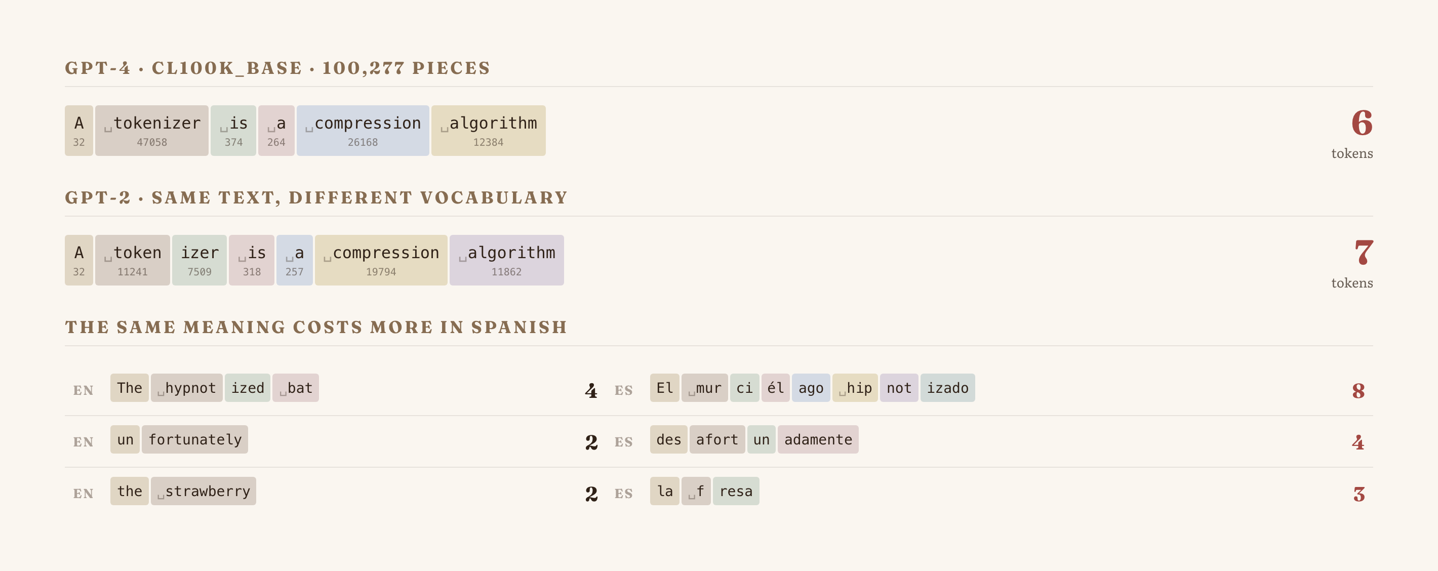
There are very good pages that explain all of it. You paste text and it shows you which tokens a production model splits it into. For example: Tiktokenizer, which lets you switch between the tokenizers of GPT-4, GPT-2, Llama and others to compare. OpenAI also has its own at platform.openai.com/tokenizer.

It's very much worth throwing weird things at it and seeing what happens. Write a word in Spanish and another in English and compare how many tokens each one uses.

Tiktokenizer splitting a phrase into colored tokens — The same algorithm with 100,277 pieces: what GPT-4 sees when you write to it.

256? bytes?

In the example above I used letters to demonstrate it in an easy way, but in the code it starts from the 256 possible bytes.

for (int i = 0; i < num_chars; i++) tokens[i] = (unsigned char)corpus[i];

Each character becomes its byte value (following ASCII). I is 73, the space is 32, a is 97. That's all there is at the beginning... 256 tokens that correspond one to one with the 256 values a byte can have.

In fact, as a curious note, in the original plan I had written down that I'd implement a special <|unk|> token for unknown words (normally LLMs do have these, to represent spaces, line breaks, when a sentence ends, a paragraph, etc...

Now with numbers

In "banana bandana" I showed the letters so it would be understandable. But inside there are no letters, there are integers, and it's worth seeing the table that actually gets computed. This is the same algorithm on "aaabdaaabac", which is the smallest text you can demonstrate anything with:

--- pass for new_id 256 ---
  pair [ 97, 97] ('aa') count=4
  pair [ 97, 98] ('ab') count=2
  pair [ 98,100] ('bd') count=1
  pair [100, 97] ('da') count=1
  pair [ 98, 97] ('ba') count=1
  pair [ 97, 99] ('ac') count=1
  => most frequent: [97,97] ('aa') x4  -> new id 256
  ids now (9): 256 97 98 100 256 97 98 97 99

--- pass for new_id 257 ---
  pair [256, 97] count=2
  pair [ 97, 98] ('ab') count=2
  pair [ 98,100] ('bd') count=1
  pair [100,256] count=1
  pair [ 98, 97] ('ba') count=1
  pair [ 97, 99] ('ac') count=1
  => most frequent: [256,97] x2  -> new id 257
  ids now (7): 257 98 100 257 98 97 99

--- learned vocabulary (merges only) ---
  vocab[256] = "aa" (len=2)
  vocab[257] = "aaa" (len=3)

initial: 11 bytes  ->  final: 7 ids

The program doesn't see text... it sees that the pair [97, 97] appears 4 times and that the pair [98, 100] appears once, and it picks the first one. The IDs are arbitrary labels, 256 doesn't mean anything other than "the first piece I learned".

In the second pass the winning pair was [256, 97], that is, the token I just invented glued to another one. 257 isn't "two bytes", it's "aa" + "a" = "aaa". That's why the vocabulary can end up containing long pieces without anyone having written them by hand.

From 11 bytes we went down to 7 IDs. That's compression and it's still a compression algorithm.

But now we have to use real text

If we run the tokenizer over a complete short story (the-verdict.txt, about 20 thousand letters) asking it for 20 merges. These are the 20 tokens it learned, without anyone programming anything about English into it:

--- the 20 merges learned from the-verdict.txt ---
  merge  0: [101, 32] -> 256   vocab[256] = "e " (len=2)
  merge  1: [ 32,116] -> 257   vocab[257] = " t" (len=2)
  merge  2: [100, 32] -> 258   vocab[258] = "d " (len=2)
  merge  3: [116, 32] -> 259   vocab[259] = "t " (len=2)
  merge  4: [105,110] -> 260   vocab[260] = "in" (len=2)
  merge  5: [115, 32] -> 261   vocab[261] = "s " (len=2)
  merge  6: [104,256] -> 262   vocab[262] = "he " (len=3)
  merge  7: [104, 97] -> 263   vocab[263] = "ha" (len=2)
  merge  8: [ 44, 32] -> 264   vocab[264] = ", " (len=2)
  merge  9: [111,117] -> 265   vocab[265] = "ou" (len=2)
  merge 10: [101,114] -> 266   vocab[266] = "er" (len=2)
  merge 11: [ 97,110] -> 267   vocab[267] = "an" (len=2)
  merge 12: [111,110] -> 268   vocab[268] = "on" (len=2)
  merge 13: [101,110] -> 269   vocab[269] = "en" (len=2)
  merge 14: [257,262] -> 270   vocab[270] = " the " (len=5)
  merge 15: [121, 32] -> 271   vocab[271] = "y " (len=2)
  merge 16: [ 46, 32] -> 272   vocab[272] = ". " (len=2)
  merge 17: [111, 32] -> 273   vocab[273] = "o " (len=2)
  merge 18: [260,103] -> 274   vocab[274] = "ing" (len=3)
  merge 19: [104,105] -> 275   vocab[275] = "hi" (len=2)

The algorithm has no concept of a "word", but it noticed that certain letters are followed by a space very frequently, and it saved that. It discovered the endings of English. "ing" was built from "in" (merge 4) plus the letter g.

With 20 merges, the 20,479 byte text was compressed to 15,881 tokens, that is 1.29x. With our model's 1,792 merges, tinyshakespeare.txt goes from 1,115,394 bytes to 359,266 tokens: 3.10x.

Model	Vocabulary size
GPT-2 / GPT-3	50,257
GPT-4 (cl100k)	100,277
Llama 3	128,256
the one we're building	2,048

Encoding

We already have the rules saved, now we need to be able to encode new text, that is, we have to apply these rules. The order must be respected. You always have to apply the merge that was learned earliest, because the late merges are built on top of the early ones. If you apply 14 before 6, 14 is never going to find its roots.

// find the pair with the lowest merge index (= learned earliest)
int best_merge = -1;
for (int i = 0; i < len - 1; i++) {
    for (int m = 0; m < num_merges; m++) {
        if (tokens[i] == merges[m].p0 && tokens[i+1] == merges[m].p1) {
            if (best_merge == -1 || m < best_merge) best_merge = m;
            break;
        }
    }
}

This is how "I HAD always thought" looks with the 276 tokenizer:

--- tokenizing "I HAD always thought" ---
  18 ids: 73 32 72 65 68 32 97 108 119 97 121 115 257 104 265 103 104 116
  id  73 -> "I"
  id  32 -> " "
  id  72 -> "H"
  id  65 -> "A"
  id  68 -> "D"
  id  32 -> " "
  id  97 -> "a"
  id 108 -> "l"
  id 119 -> "w"
  id  97 -> "a"
  id 121 -> "y"
  id 115 -> "s"
  id 257 -> " t"   <- learned merge
  id 104 -> "h"
  id 265 -> "ou"   <- learned merge
  id 103 -> "g"
  id 104 -> "h"
  id 116 -> "t"

20 letters, 18 tokens. Almost nothing got compressed, and the capitals (I, H, A, D) were left loose as individual bytes, because capitals are rare in the corpus and never won a merge.

And now the same thing with the real 2,048 tokenizer:

merges loaded: 1792  (vocab_size = 2048)

"I HAD always thought"
  -> 8 tokens: 313 72 1054 2041 1165 259 376 802
  -> pieces: |I |H|AD| al|way|s |thou|ght|

From 18 tokens to 8. "AD" is a single token, "thou" is a single token. That "thou" exists because the corpus is Shakespeare and there thou shows up every three lines. The vocabulary is a statistical portrait of the corpus. A tokenizer trained on Shakespeare and one trained on Python code split the same text in completely different ways.

Which becomes much more obvious with a line taken from the corpus itself:

"First Citizen:
Before we proceed any further, hear me speak."
  -> 17 tokens
  -> pieces: |First |Citizen:\n|Be|fore |we |pro|c|eed |any |f|ur|ther|, |hear| me |speak|.|

|Citizen:\n|, a single token containing a word, a colon and a line break. The tokenizer didn't learn the word "Citizen", it learned the formatting pattern of a play script, because in tinyshakespeare.txt that exact combination shows up constantly. To the model, "Citizen followed by a colon followed by a line break" is one unit, similar to the letter a.

As a curious note, that's why, when you ask an LLM how many r's "strawberry" has, the model never saw the letters. It saw two or three numbers. You're asking it about something that was destroyed before the model started to exist.

Decoding

Decoding is the opposite. Each ID knows which bytes it expands to, so you glue the bytes and that's it. Since each token is deep down a list of bytes, the encode → decode cycle is exact.

It's worth noting that in the vocabulary I don't save text, I save raw bytes:

typedef struct {
    int id;                 // key (0..vocab_size-1)
    unsigned char *bytes;   // raw bytes this id expands to
    int len;                // length of bytes
    UT_hash_handle hh;
} Vocab;

With unsigned char * and an explicit length, not with a char * terminated in \0. If I used C strings, a token containing a zero byte would break everything, and in a byte level vocabulary the zero token exists by definition.

Decoding is two parts. One to measure how much the result is going to weigh, and another to copy the bytes:

char *decode(const int *ids, int ids_len, Vocab *vocab) {
    int total = 0;
    for (int i = 0; i < ids_len; i++) {
        Vocab *v;
        HASH_FIND_INT(vocab, &ids[i], v);
        total += v->len;
    }

    char *out = malloc(total + 1);
    int pos = 0;
    for (int i = 0; i < ids_len; i++) {
        Vocab *v;
        HASH_FIND_INT(vocab, &ids[i], v);
        memcpy(out + pos, v->bytes, v->len);
        pos += v->len;
    }
    out[total] = '\0';
    return out;
}

Table lookups and memcpy. And I think it's worth explaining this, because this function is the one that produces the text that comes out of an LLM. Everything you read on the screen when you talk to ChatGPT comes out of something very close to these lines. A memcpy of bytes that somebody saved in a hashmap. All the difficulty was in choosing the IDs.

The dataloader

We already have a long list of numbers. 359,266 tokens. But that isn't a training set. You have to split it into examples, and each example needs a question and an answer. This has to do with how deep learning works, but I'm not going to explain it in this blog :).

tensor_set(&inputs,  (int[]){x, y}, tokens[x * STRIDE + y]);
tensor_set(&targets, (int[]){x, y}, tokens[x * STRIDE + y + 1]);

inputs is a window of the text, targets is the same window shifted one to the right. Given what you have so far, predict the next token. That's why it can only predict one token at a time, and when you see ChatGPT loading the tokens, it does them as if it were typing.

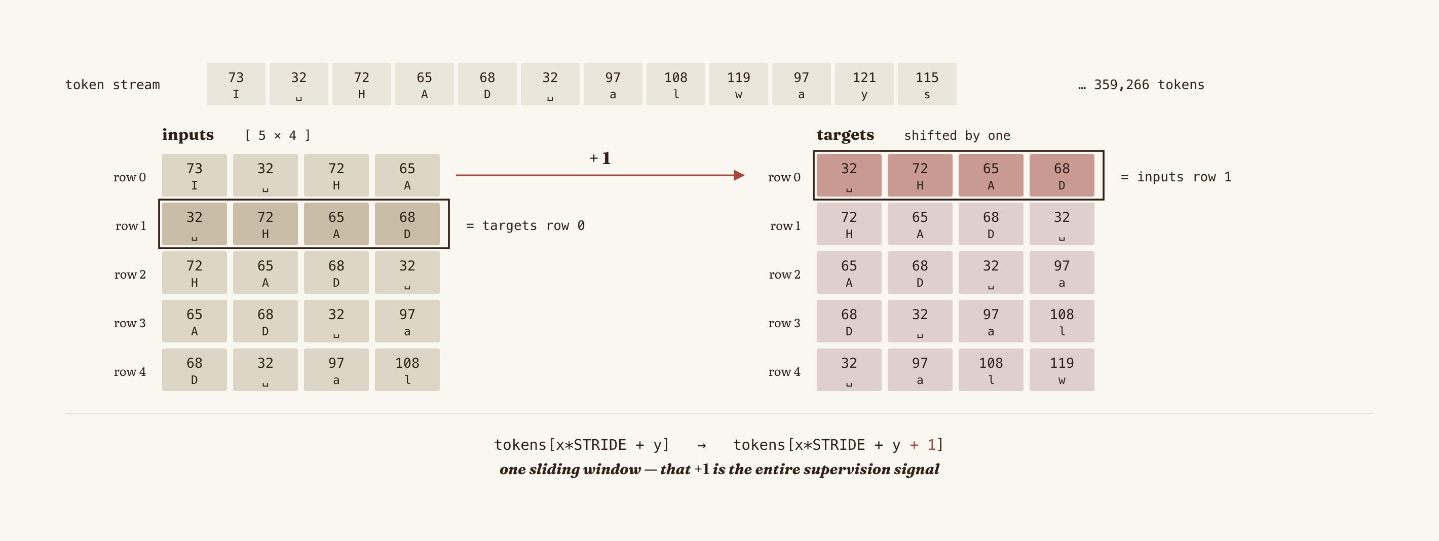
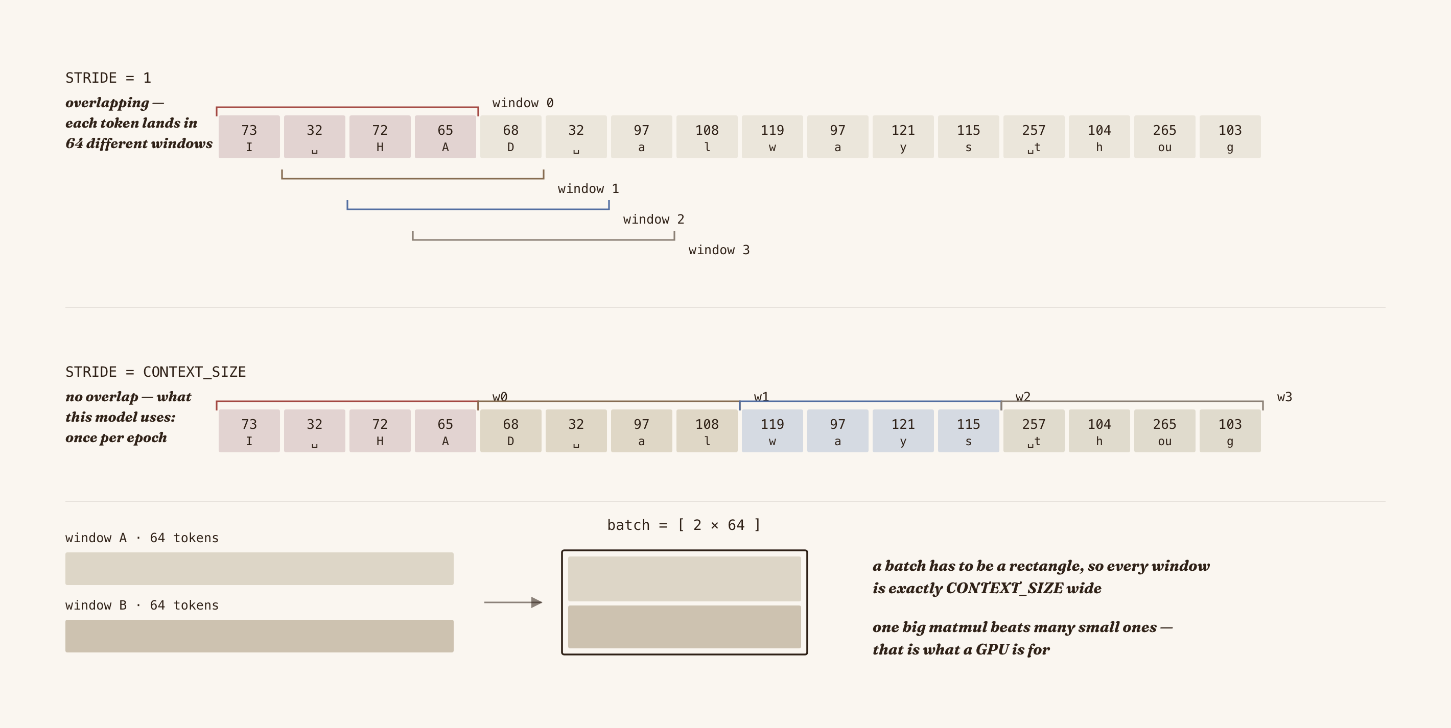
Inputs and targets: the same token sequence shifted one place to the right — The targets are the inputs shifted one place. All the supervision is right there.

With windows of 4 tokens and stride 1:

enc_sample (first 20 of 15881 tokens):
  [ 73 32 72 65 68 32 97 108 119 97 121 115 257 104 265 103 104 259 74 97 ]

inputs (2D tensor, showing first 5 rows, CONTEXT_SIZE=4, STRIDE=1):
  row 0: [   73   32   72   65 ]
  row 1: [   32   72   65   68 ]
  row 2: [   72   65   68   32 ]
  row 3: [   65   68   32   97 ]
  row 4: [   68   32   97  108 ]

targets (2D tensor, showing first 5 rows, shifted by +1):
  row 0: [   32   72   65   68 ]
  row 1: [   72   65   68   32 ]
  row 2: [   65   68   32   97 ]
  row 3: [   68   32   97  108 ]
  row 4: [   32   97  108  119 ]

If we compare inputs row 0 with targets row 0. It's the same sequence, shifted one. And inputs row 1 is targets row 0. It's a window sliding over the text.

Normal supervised learning needs a human to label data:. That is, somebody has to mark ten thousand photos as "cat" or "dog". Here the labels already came inside the text. Every position of every sentence on the internet is a labeled example and the label is simply the word the author wrote after it. We gave the training data to the LLMs. That's why it's called self-supervised, and that's why it could be scaled to trillions of tokens.

All of an LLM's knowledge comes from that single task repeated a whole lot of times. Guess the next word.

The STRIDE controls how much the window moves:

// stride == context_size  ->  non-overlapping windows (typical real training)
// stride <  context_size  ->  overlapping windows (more data, redundancy)
// stride == 1             ->  every position is a window start (didactic setup)

With stride 1 every position starts a window, which is perfect for seeing the effect in the console... but, the same token shows up in 64 different windows. Our model uses stride 64 with a window of 64, that is, windows that don't overlap, each token is seen once per epoch.

The batch. Instead of giving the model one window at a time, you give it several and it processes them all together in the same operation. If you stack 2 windows of 64 tokens you have a batch of size 2, that is, a table of $2 \times 64$ .

It's done for two reasons. One is speed... multiplying one big matrix in one shot is much faster than multiplying several small ones, which is exactly what GPUs are for. The other is stability... if you correct the model with a single example, every correction is going to be contaminated by however weird that particular example is. If you average the error of several, the correction points in a more reliable direction.

a batch is a rectangle. To stack two sequences they have to measure exactly the same. You can't stack one of 40 tokens with one of 64. That's why the dataloader produces windows of fixed width, and that's why that width is CONTEXT_SIZE.

Sliding window over the token sequence, with inputs and targets offset by one — The stride decides how much the window moves; the batch turns it into a rectangle.

In the model we're building, I did something wrong. My dataloader materializes all the windows in memory at once, and that doesn't scale.

/* Note: in a real foundational model, the dataloader does not materialize
   every sliding window up front. With STRIDE=1, CONTEXT_SIZE=256 and a
   5000-token corpus you get ~4744 windows * 256 floats * 4 bytes ~= 4.8 MB
   for inputs and another 4.8 MB for targets, before the embedding layer even
   runs. At billions of tokens that is impossible.
   Instead, store only the token stream + an array of starting indices
   (num_windows * 4 bytes, tiny) and assemble x/y batches on the fly ...
   Shuffle the indices (Fisher-Yates), not the data. This is what PyTorch's
   DataLoader does under the hood. */

The problem is that I'm saving the same token 64 times. A corpus of 5,000 tokens turns into 9.6 MB of windows. Scaling that to the trillions of tokens a production model is trained on, you'd need more hard drive than exists.

But we solve it by saving only the strip of tokens and an array of starting indices. Window $k$ is assembled on the spot by reading from idx[k]. And to shuffle the data between epochs, you don't shuffle the text, you shuffle the indices (with Fisher-Yates, which is a permutation in linear time). It's what PyTorch's DataLoader does, and it's the reason you can train with a dataset bigger than your RAM.

I didn't implement it because with tinyshakespeare the 9 MB fit and I wanted to keep moving.

Here it is in full:

DataLoader create_dataloader_v1(int *tokens, int num_tokens) {
    const int num_windows = ((num_tokens - 1 - CONTEXT_SIZE) / STRIDE) + 1;

    const int shape[2] = {num_windows, CONTEXT_SIZE};
    Tensor inputs = tensor_create(shape, 2);
    Tensor targets = tensor_create(shape, 2);

    for (int x = 0; x < num_windows; x++) {
        for (int y = 0; y < CONTEXT_SIZE; y++) {
            tensor_set(&inputs,  (int[]){x, y}, tokens[x * STRIDE + y]);
            tensor_set(&targets, (int[]){x, y}, tokens[x * STRIDE + y + 1]);
        }
    }

    DataLoader loader;
    loader.inputs = inputs;
    loader.targets = targets;

    return loader;
}

That + 1 on the last line of the loop is the entire supervised learning of the model. And the - 1 on the first line exists so the last window still has a next token to predict.

Embeddings

A token ID is a number, but it's a number with no arithmetic meaning. Token 270 is " the " and token 271 is "y ". Is 270 less than 271? Numerically yes, but that doesn't mean anything. Does 270 + 1 = 271 mean that " the " plus something gives "y "? Obviously not. IDs are labels, they're names, not quantities. They can't be added or multiplied or averaged.

And the problem is that multiplying and adding is the only thing the neural network knows how to do.

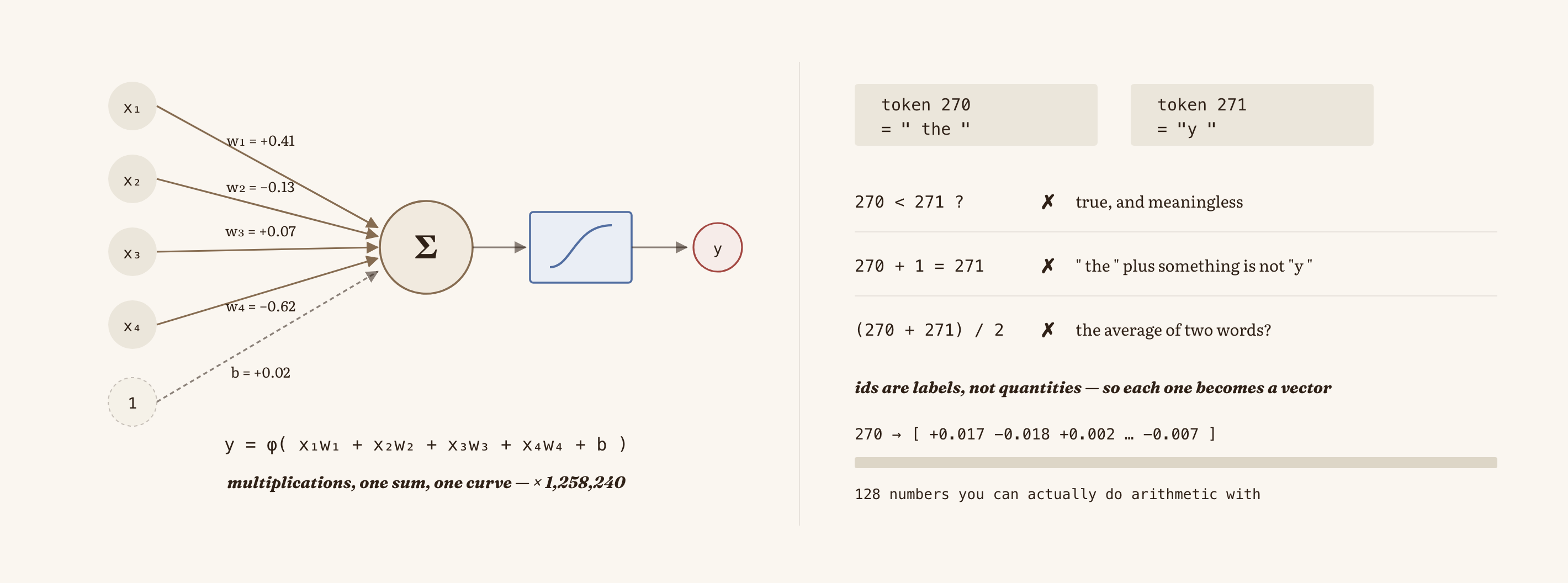
Close-up of an artificial neuron: inputs multiplied by weights and summed — Multiply and add. That's why a token ID can't go in directly.

So we have to turn each label into something you can actually do arithmetic with... a vector. That's what's called an embedding, and the implementation is a lookup table. A matrix with one row per token:

const int tok_emb_shape[2] = {cfg->vocab_size, cfg->emb_dim};
self->tok_emb = tensor_create_random(tok_emb_shape, tok_emb_dim, 0.02);

In our model that's a matrix of $2048 \times 128$ . Each one of the 2,048 tokens has 128 numbers describing it. So we can actually see it, we're going to do it as $276 \times 16$ :

Token embedding layer [276 x 16] (random init, scale=0.02):
  (showing first 10 rows)
  tok   0: [ +0.017 -0.018 +0.002 -0.007 -0.007 -0.012 +0.007 +0.001 ... ]
  tok   1: [ -0.013 +0.007 -0.012 -0.001 -0.005 +0.008 +0.009 -0.016 ... ]
  tok   2: [ -0.006 +0.012 +0.020 +0.009 -0.006 +0.007 -0.001 -0.004 ... ]
  tok   3: [ +0.007 -0.010 +0.009 -0.000 -0.007 +0.010 +0.019 -0.002 ... ]
  ...

They're random numbers. There's no meaning there yet, it's noise. That matrix is one of the parameters training is going to modify, and the meaning of words is going to emerge inside it by correcting prediction errors. The model doesn't start out knowing what a word is, it starts with noise and arranges it. Also, about parameters and training them, those are deep learning topics we're not going to touch here.

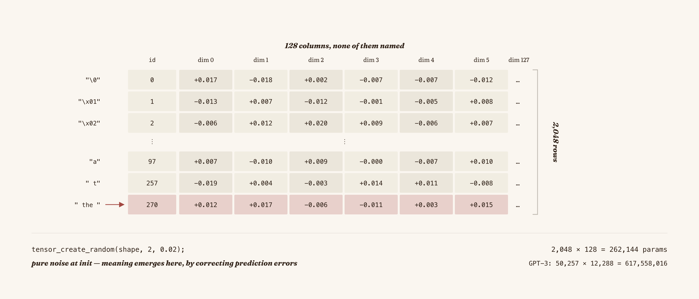
The embedding matrix as a lookup table: one row of numbers per token — A lookup table of 2,048 × 128 that starts out as pure noise.

The 128 columns have no names. I wrote that matrix and I have no idea what column 47 represents. There's no "is a noun" column or an "is positive" one. They're 128 directions (or dimensions) the model chose on its own only because they helped it lower the error. This is exactly what I said in the introduction about Deep Learning... the machine doesn't only find the rules, it also decides what the features are. It's not that someone is hiding the information from us, it's that the information was never in words.

Why 128 and not 12,288 like GPT-3:

#define EMBEDDIGS_OUTPUT_DIM 16 // a tiny vocabulary doesn't need a huge embedding
                                                                    // space to represent distinctions between tokens

The embedding size is how much room you give the model to distinguish tokens. With 2,048 tokens, 128 dimensions is nothing. GPT-3 needs 12,288 because it has to fit 50,257 tokens and capture much finer distinctions between them.

The position problem

We're missing something. Token embeddings give us the what, but not the where.

This is a problem because the transformer doesn't use recurrence. An RNN knew the order because it literally read in order, position was implicit in time. Attention looks at all positions at the same time (we're going to see that below), and that's its big advantage, but the cost is that it has no sense of order at all. To pure attention, "the dog bites the man" and "the man bites the dog" are the same set of tokens.

The solution is a second table, indexed by position instead of by token:

Positional embedding layer [4 x 16] (random init, scale=0.02):
  pos 0: [ -0.008 +0.016 -0.018 +0.015 +0.016 +0.010 -0.003 +0.008 ... ]
  pos 1: [ -0.001 +0.010 +0.005 -0.008 +0.012 -0.015 -0.006 +0.020 ... ]
  pos 2: [ -0.012 +0.010 +0.015 +0.019 +0.009 -0.015 +0.020 -0.013 ... ]
  pos 3: [ +0.015 +0.006 -0.012 +0.005 +0.007 +0.009 +0.017 -0.005 ... ]

It's a matrix of $[\text{window} \times \text{dimension}]$ . One learned vector for "being at position 0", another for "being at position 1". Just like the token ones... they start as noise and training gives them meaning.

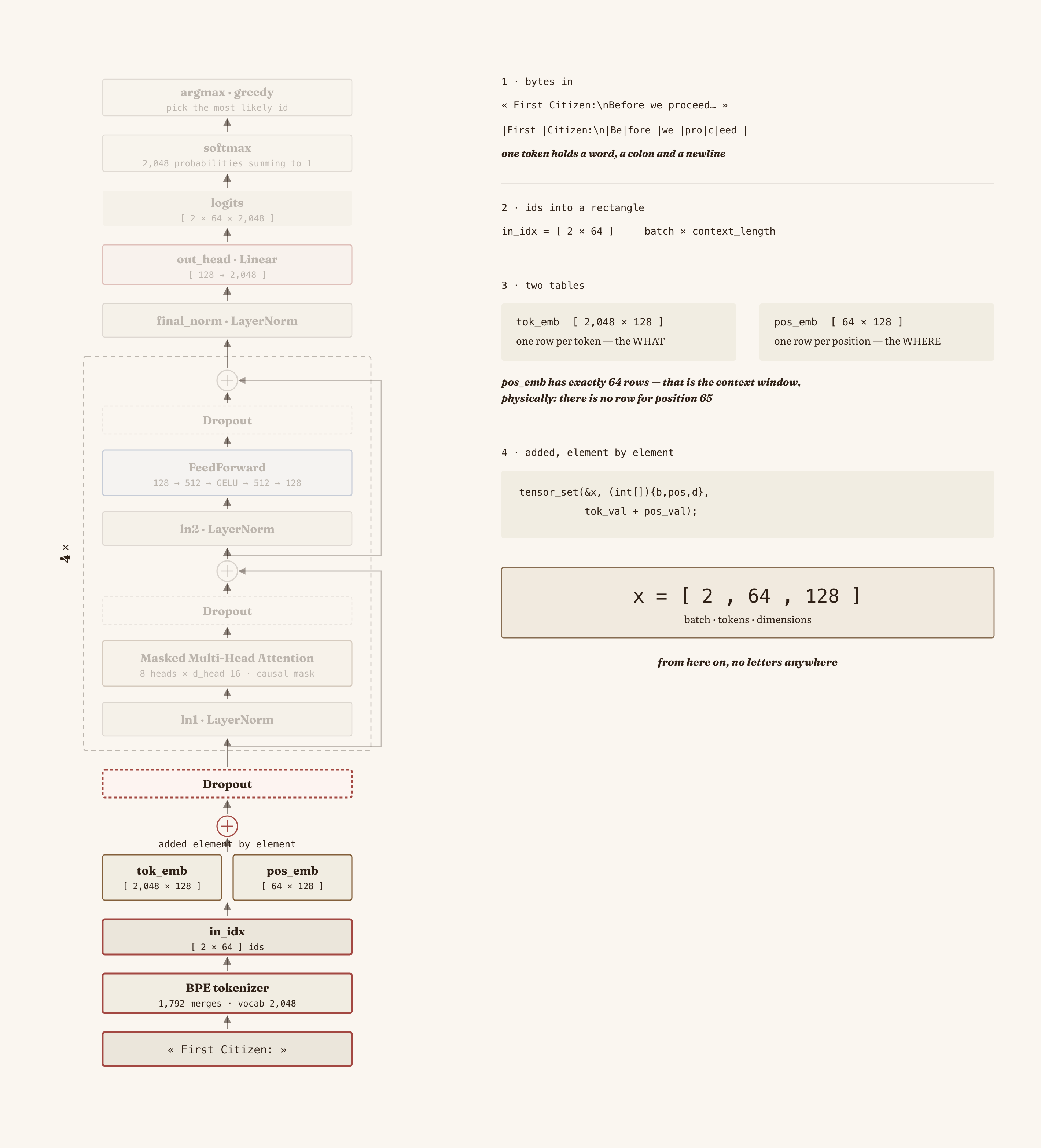
We can see that this table has exactly 64 rows, not one more. That's the real, physical reason a model has a limited context window. There is no row for position 65. It's not a software restriction, it's that the matrix runs out.

Now, we just have to add

The two vectors get added. And this is the complete block, which is literally the first thing the model does when you run it:

Tensor x = tensor_create(x_shape, x_dim);   // [batch, tokens, emb_dim]

for (int b = 0; b < batch_size; b++) {
    for (int pos = 0; pos < seq_len; pos++) {

        const int coords_x[2] = {b, pos};
        int token_id = (int)tensor_get(&in_idx, coords_x, 2);

        for (int d = 0; d < cfg->emb_dim; d++) {
            // fetch from token embedding matrix
            const int tok_coords[2]  = {token_id, d};
            float tok_val = tensor_get(&self->tok_emb, tok_coords, 2);

            // fetch from positional embedding matrix
            const int pos_coords[2]  = {pos, d};
            float pos_val = tensor_get(&self->pos_emb, pos_coords, 2);

            // token_emb + pos_emb = input_emb
            const int out_coords[3] = {b, pos, d};
            tensor_set(&x, out_coords, tok_val + pos_val);
        }
    }
}

Element by element. One plus the other.

Two random vectors in a high dimensional space are almost perpendicular to each other. The sum lives in a space so large that the following layers can learn to separate the contribution of each part by projecting onto the right directions. The position information and the identity information end up in practically independent subspaces.

This is the sum:

Input embeddings [3970 x 4 x 16] = token_emb + pos_emb:
  (showing window 0, all 4 positions)
  pos 0: [ -0.025 +0.031 -0.013 +0.027 +0.036 ... ], token_id (73) # I
  pos 1: [ +0.012 +0.016 -0.013 -0.015 +0.022 ... ], token_id (32) #
  pos 2: [ -0.025 +0.016 +0.034 +0.010 +0.022 ... ], token_id (72) # H
  pos 3: [ +0.033 +0.016 -0.011 -0.007 +0.024 ... ], token_id (65) # A

From here on there are no letters. There's a matrix of $[\text{batch} \times 64 \times 128]$ and nothing else, until the end of the model where it gets turned back into tokens.

The text is gone. What's left is this:

[\,\underbrace{2}_{\text{batch}},\ \underbrace{64}_{\text{tokens}},\ \underbrace{128}_{\text{dimensions}}\,]

How many examples we're processing at once, how many tokens each one has, and how many numbers describe each token. Those three dimensions are what we're going to use for what comes next.

Everything that follows (attention, the 4 layers, generation) operates on this same thing. The next question is how those points start looking at each other, and that's the attention mechanism.

First part of the GPT architecture: from text to the input embeddings — From text to the input embeddings. From here on there are no letters.

The attention mechanism

We already have a tensor of $[2, 64, 128]$ . Each token turned into a point in a 128 dimensional space. But a problem comes up here, and it's that it doesn't depend on context.

The word "bank" has one single row in the embedding matrix. The exact same vector for "I sat on the bank of the river" and for "I went to the bank to take out money". The model is incapable of telling them apart, because the vector is looked up by token ID only.

The cat that was on the roof came down because it was hungry.

Who was hungry? To answer that you have to link "it" with "cat", which is seven words back, skipping over "roof" which is closer but isn't the subject. No amount of information inside the vector of "it" can solve that, because the answer isn't in "it", it's in another part of the sentence.

So we need a mechanism that lets each token look at the others and rewrite itself with what it found. That's what we call attention.

Simpler

Imagine each token in the sentence is a person in a room, and they can all see each other.

Each person asks the same question at the same time: "which of the people here matters to me for understanding what I am?"

Everyone gives a score to everyone else. The word "it" scores "cat" high and "roof" low. Afterwards, each person keeps a summary... a mixture of everyone else, where each one contributes in proportion to the score it was given.

And here's the important part. At the end of the process, each token rewrites itself. The vector of "it" stops being the generic vector of the word "it" and becomes the vector of "it, referring to a cat, in a sentence about hunger". It came in as a dictionary word and came out as a word in a context.

Step 1: measure similarity with the dot product

We need a way to score how much one token matters to another. Tokens are vectors, so the question is, how do you measure how similar two vectors are?

The dot product. You multiply the vectors element by element and sum everything.

\omega_{ij} = x_i \cdot x_j = \sum_{d} x_i[d] \cdot x_j[d]

float dot_product(float v[], float u[], int n) {
    float result = 0.0;
    for (int i=0; i<n; i++) {
        result += v[i] * u[i];
    }
    return result;
}

And it works very well because the dot product is large when the two vectors point in the same direction, is zero when they're perpendicular, and is negative when they point in opposite directions. If two tokens ended up in the same region of the 128 dimensional space, their dot product is high. If they ended up in different regions, it's low.

That number is what we call the attention score, and they're computed all against all. With 4 tokens that's 16 scores, that is, a $4 \times 4$ matrix. With 64 tokens it's 4,096.

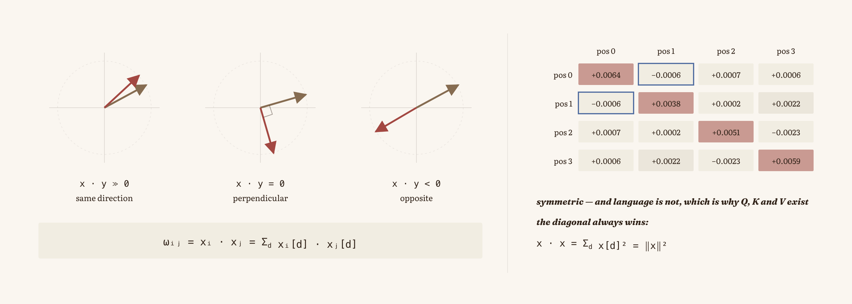
The dot product as a similarity measure: aligned, perpendicular and opposite vectors — The dot product as a similarity measure, and the matrix that comes out of it.

This is how the matrix computed over the embeddings with a window of 4 tokens ("I", " ", "H", "A") looks:

Attention scores [3970 x 4 x 4] (showing window 0, raw dot products before softmax):
            pos 0    pos 1    pos 2    pos 3
  pos 0:  +0.0064 -0.0006 +0.0007 +0.0006
  pos 1:  -0.0006 +0.0038 +0.0002 +0.0022
  pos 2:  +0.0007 +0.0002 +0.0051 -0.0023
  pos 3:  +0.0006 +0.0022 -0.0023 +0.0059

The row is who's asking, the column is who's being asked. The row pos 0 says how much each of the four tokens matters to "I".

It's symmetric: the value at (0,1) is $-0.0006$ and the one at (1,0) too. It has to be that way, because $x_0 \cdot x_1$ and $x_1 \cdot x_0$ are the same multiplication. This is the reason we're going to need three matrices instead of zero further down. If similarity is symmetric, then "cat matters to me" and "I matter to cat" are necessarily equal, and in language that's false.

The diagonal always wins: $0.0064$ , $0.0038$ , $0.0051$ , $0.0059$ on the diagonal, against values of $\pm 0.002$ everywhere else. In all four rows, the biggest number is the one on the diagonal.

The dot product of a vector with itself is:

x \cdot x = \sum_d x[d]^2 = \|x\|^2

A sum of squares, which means it can never be negative, and it's always greater than or equal to the dot product with any other vector of similar norm.

Step 2: from scores to weights with softmax

The scores are strange numbers... there are negatives, there are positives, and they don't add up to anything in particular. To mix we need proportions: numbers between 0 and 1 that add up to exactly 1, so we can say "70% comes from cat and 30% from roof".

That's what softmax does:

a_{ij} = \frac{e^{\omega_{ij}}}{\sum_k e^{\omega_{ik}}}

You raise $e$ to each score and divide by the sum of all of them.

Applied to the matrix above:

Attention weights [3970 x 4 x 4] (showing window 0, post-softmax):
            pos 0    pos 1    pos 2    pos 3      sum
  pos 0:  +0.2512 +0.2494 +0.2497 +0.2497   1.000000
  pos 1:  +0.2495 +0.2506 +0.2497 +0.2502   1.000000
  pos 2:  +0.2499 +0.2498 +0.2511 +0.2492   1.000000
  pos 3:  +0.2497 +0.2502 +0.2490 +0.2511   1.000000

Each row adds up to 1. Now we do have proportions.

Softmax blows up if you write it exactly as the formula says

PyTorch solves it. But in C it's different.

// in real production code, use PyTorch's built-in softmax for numerical stability.
void softmax(float *input, int size) {
    // subtract max for numerical stability: shift-invariant, prevents expf overflow
    float max = input[0];
    for (int i = 1; i < size; i++) if (input[i] > max) max = input[i];
    float sum = 0.0;
    for (int i = 0; i < size; i++) {
        input[i] = expf(input[i] - max);
        sum += input[i];
    }
    for (int i = 0; i < size; i++) {
        input[i] /= sum;
    }
}

The problem is expf. A 32 bit float goes up to $3.4 \times 10^{38}$ , and $\ln(3.4 \times 10^{38}) \approx 88.7$ . Which means expf(89) is already infinity. And as soon as you have an infinity in the numerator and another in the denominator, the division gives you NaN, and the NaN spreads to the whole model in the next matmul.

So, we have to subtract the maximum from all the scores before exponentiating. And it's valid because subtracting a constant doesn't change the result, it cancels out above and below:

\frac{e^{x_i - c}}{\sum_k e^{x_k - c}} = \frac{e^{x_i} \cdot e^{-c}}{e^{-c}\sum_k e^{x_k}} = \frac{e^{x_i}}{\sum_k e^{x_k}}

Step 3: the context vector

With the weights we can now mix. The context vector of a token is the sum of all the vectors, each one multiplied by its weight:

z_i = \sum_j a_{ij} \cdot x_j

And since the weights are already in one matrix and the vectors in another, that entire sum is a single matrix multiplication:

Tensor context_vectors = tensor_matmul(&attention_weights, &input_embeddings);

Context vectors [3970 x 4 x 16] = attention_weights @ input_embeddings:
  (showing window 0, all 4 positions)
  pos 0: [ -0.00127 +0.01974 -0.00074 +0.00369 +0.02606 +0.00016 ... ]
  pos 1: [ -0.00120 +0.01972 -0.00074 +0.00362 +0.02604 +0.00017 ... ]
  pos 2: [ -0.00128 +0.01973 -0.00068 +0.00367 +0.02605 +0.00010 ... ]
  pos 3: [ -0.00116 +0.01972 -0.00077 +0.00362 +0.02605 +0.00022 ... ]

The four rows are almost identical. If the weights are all $0.25$ , then the four tokens are computing the same average of the same four vectors. Four different tokens went in and four copies of the same thing came out.

Untrained attention destroys information. It flattens the four tokens into their average and erases the differences between them.

Query, Key and Value

Attention doesn't compare the tokens directly, instead it first projects them into three different spaces, each one with its own trainable weight matrix:

q_i = x_i W_q \qquad k_i = x_i W_k \qquad v_i = x_i W_v

void MultiHeadAttention_init(MultiHeadAttention *self, GPT_CONFIG *cfg) {
    const int weight_matrices_shape[2] = {cfg->emb_dim, cfg->emb_dim};
    self->W_query = tensor_create_random(weight_matrices_shape, 2, 0.02);
    self->W_key   = tensor_create_random(weight_matrices_shape, 2, 0.02);
    self->W_value = tensor_create_random(weight_matrices_shape, 2, 0.02);
}

Three $128 \times 128$ matrices per block. They start as noise, just like everything else, and they're among the parameters training is going to modify.

Why three?

query is what you're looking for. You get to the counter and say "I want something about cats".
key is what each book announces about itself. The title. It's what gets compared against your search.
value is what the book actually contains. It's what you take with you.

The matching is done with queries against keys, but what gets transported are the values. Q/K for the matching, V to bring the content.

Why does V have to be different from K? Because what makes you findable isn't the same as what you contribute. A book titled "Cats" is easy to find by searching "cats", but what it contributes is 300 pages of content, not the word in the title. In language it's the same. If we used the same vector for both things, the model would have to choose between being findable or being useful. With two matrices it can be both.

And here the symmetry problem we saw a while ago also gets fixed. The scores are no longer $x_i \cdot x_j$ , they're:

\omega_{ij} = q_i \cdot k_j = (x_i W_q) \cdot (x_j W_k)

Which is no longer symmetric, because $q_i \cdot k_j$ goes through $W_q$ and $W_k$ , while $q_j \cdot k_i$ goes through the same matrices but flipped. The relationship has direction, which is what language needs.

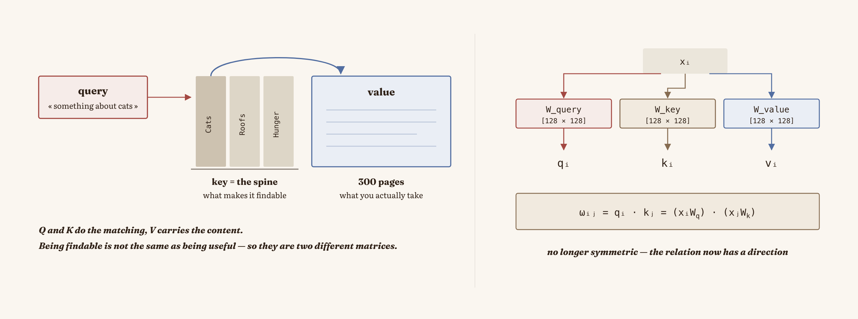
Query, key and value: the search, the title on the spine, and the content of the book — The search, the spine of the book and its content: three projections of the same token.

And the matrix of all the scores comes out of a transpose and a matmul.

// attention scores from queries @ keys^T.
// matmul over (i,j) is exactly q_i · k_j packed as a matrix:
//   S[i,j] = Σ_d Q[i,d] * K[j,d]  ==  q_i · k_j
// transpose puts d_out on the inner axis so matmul contracts the right dim.
Tensor keys_T = tensor_transpose(&keys);
Tensor attention_scores_2 = tensor_matmul(&queries, &keys_T);

The `grad` field that isn't useful for anything yet

When I defined the tensor, I gave it a field we've never used until now:

typedef struct {
    float *data;
    int *shape;
    int *strides;
    int ndim;
    int size;
    float *grad;    // <- this one
} Tensor;

In PyTorch this is requires_grad=True. It's the space where, for each of the tensor's numbers, how much it would have to move for the model to be less wrong is going to be saved.

Right now it's NULL for everything. The three $W$ matrices exist, they get used, and they're completely useless... they're random noise that never gets corrected. All of this describes a machine that learns nothing. Later, we're going to train the model and that value is going to make sense.

The scale

Before softmax there's an important step we have to do. The scores get divided by the square root of the dimension:

a_{ij} = \text{softmax}\!\left(\frac{q_i \cdot k_j}{\sqrt{d_k}}\right)

const float scale_mh = 1.0f / sqrtf((float)d_head);

/*
    the reason for normalization by embedding size is to improve the training
    performance by avoiding small gradients. As dot products increase, the softmax
    function behaves more like a step function, resulting in gradients nearing zero...

    the scaling by the square root of the embedding dimension is the reason why this self-attention mechanism is also called scaled-dot product attention.
*/

A dot product is a sum of $d$ terms. If the components of the vectors are independent and of similar variance, the variance of the sum grows proportional to $d$ , and therefore the standard deviation grows with $\sqrt{d}$ . Which means the bigger you make the model, the bigger the scores get just from having more terms to add up.

And softmax with big numbers saturates. If you give it $[1, 2, 3]$ it hands out something like $[0.09, 0.24, 0.67]$ . If you give it $[10, 20, 30]$ it hands out $[0.000, 0.000, 1.000]$ . It stops being a smooth split. The maximum takes everything and the rest go to zero. A disaster for training, because the derivative of a flat function is zero. If softmax already decided $[0, 0, 1]$ , moving the weights a little doesn't change the result, and if the result doesn't change there's no gradient, and without a gradient there's no learning.

Dividing by $\sqrt{d_k}$ helps us cancel that growth and keeps the scores in a range where softmax is still a curve and not a step. And that's where the name of the mechanism comes from, "scaled dot-product attention".

Casual mask

As it stands, each token sees all the others, including the ones ahead. And remember the task is to predict the next token.

So if the token at position 3 can look at position 4, we're asking it to guess token 4 while letting it read token 4. That's called information leakage.

At generation time the future doesn't exist. You're producing one token at a time, there's nothing to the right to copy. A model trained with leakage learns to cheat on an exam where the answers are there, and then you put it in the real exam where they aren't.

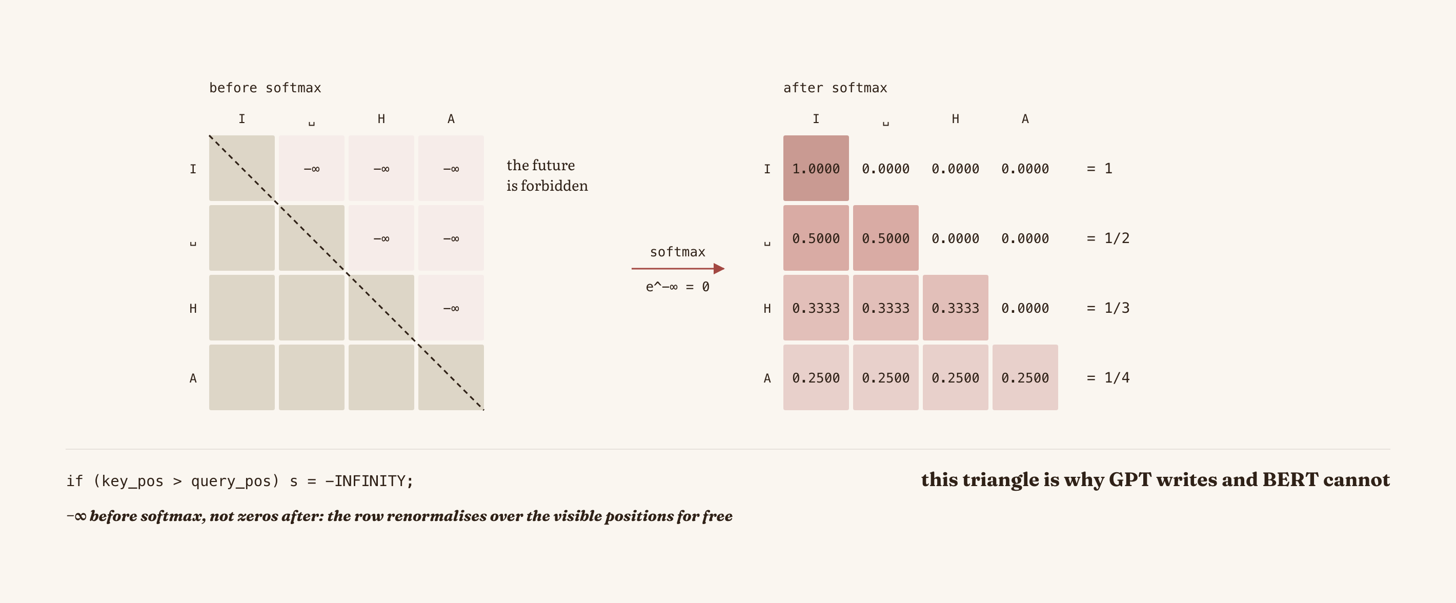
The causal mask: lower triangle allowed, upper triangle forbidden — The triangle that lets GPT write and not BERT.

The intuitive way to fix it is to compute softmax normally and then set to zero everything above the diagonal. The problem is that by killing those values, the rows no longer add up to 1, so you have to renormalize by dividing each row by its new sum.

But there's a better way... Instead of erasing it after softmax, we put $-\infty$ before:

float s = tensor_get(&attention_scores_mh, coords, 3) * scale_mh;
if (key_pos > query_pos) s = -INFINITY;  // causal mask
row_buffer_mh[key_pos] = s;

$e^{-\infty} = 0$

// causal mask: a query at query_pos may not attend to future keys.
// set them to -inf *before* softmax so expf(-inf)=0 and the row
// renormalizes over only the visible (key_pos <= query_pos) positions.

The numerator of the forbidden positions is zero, so they contribute nothing to the sum in the denominator, so softmax already normalizes over the visible positions only.

Causal attention weights [3970 x 4 x 4] (showing window 0, masked softmax, d_k=16):
            pos 0    pos 1    pos 2    pos 3      sum
  pos 0:  +1.0000 +0.0000 +0.0000 +0.0000   1.000000
  pos 1:  +0.5000 +0.5000 +0.0000 +0.0000   1.000000
  pos 2:  +0.3333 +0.3333 +0.3333 +0.0000   1.000000
  pos 3:  +0.2500 +0.2500 +0.2500 +0.2500   1.000000

$1$ , $\frac{1}{2}$ , $\frac{1}{3}$ , $\frac{1}{4}$ .

This triangle is also technically the answer to the question of why GPT can write and BERT can't.

Dropout

There's one more step that only exists during training. Throwing away a part of the weights, at random.

Tensor tensor_create_dropout(const int *shape, const int ndim, const float rate) {
    Tensor t = tensor_create(shape, ndim);
    const float keep_scale = 1.0f / (1.0f - rate);

    for (int i = 0; i < t.size; i++) {
        float r = (double) rand() / RAND_MAX;
        t.data[i] = (r > rate) ? keep_scale : 0.0f;
    }

    return t;
}

A mask of the same size is built where each position is 0 (with probability rate) or keep_scale (with the rest), and it gets multiplied element by element.

Why do we break the model? Because it prevents the model from depending on a single path.

If a specific connection turns out to be very useful, the network is going to lean on it more and more, until its prediction depends on that connection being there. That works perfectly for the training text and fails for new text, because what it memorized was a quirk of its data, not a rule of the language. That's overfitting.

With dropout, no connection can count on existing. At each step a different part disappears at random, so the network is forced to store the same information in several places.

This is the mask at 10%:

After dropout (rate=0.10) [3970 x 4 x 4] (showing window 0; ~10% zeroed, survivors x1.11):
            pos 0    pos 1    pos 2    pos 3      sum
  pos 0:  +0.0000 +0.0000 +0.0000 +0.0000   0.000000
  pos 1:  +0.5556 +0.5556 +0.0000 +0.0000   1.111111
  pos 2:  +0.3704 +0.3704 +0.3704 +0.0000   1.111111
  pos 3:  +0.2778 +0.2778 +0.2778 +0.2778   1.111111

The rows no longer add up to 1, they add up to 1.111. That's normal, because what dropout preserves is the expected value, not the sum of each individual row. If you averaged many different masks, the average would come out at 1.

And row 0 adds up to zero. That token was left out. That's normal too.

In the final configuration of our model dropout is off.

cfg.drop_rate = 0.0f;

I implemented it, it works, and I left it at zero because with 1.26 million parameters and a corpus of a single Shakespeare book, the model has other problems much bigger than overfitting from excess capacity. We're going to see it further down.

Multi-head

Something else is missing. Everything I described so far is one attention head, and one head has a limitation... for each token it produces a single distribution of weights, which means it can express only one type of relationship at a time.

But language has many simultaneous relationships. So we need to run several heads in parallel, each with its own criterion, and put the results together. Our model has 8.

The obvious thing is to have 8 independent attention modules, run them in a for and concatenate the outputs. It's perfectly understandable, in fact, that's how I implemented it the first time...

The problem isn't the number of arithmetic operations, which is almost the same. The problem is that eight small multiplications are much slower than one big one, even if they do the same number of multiplications. For three reasons:

In a small matrix, the time gets eaten by bringing the data from RAM to the cache, not by multiplying. A big operation amortizes that trip across many more computations.
A GPU has thousands of cores. A $16 \times 16$ matrix isn't enough to occupy them, so most of them sit waiting.
Launching the work, synchronizing, waiting.

The efficient way

The trick is realizing that the three $W$ matrices are already big enough for all the heads.

$W_q$ is $128 \times 128$ , and $128 = 8 \times 16$ . So the 128 output columns already are, if you want to see it that way, the 16 columns of head 0, followed by the 16 of head 1, and so on up to 8. There's nothing to split. A single multiplication of $[T, 128] \times [128, 128]$ has already computed the projections of the eight heads. The only thing left is to reinterpret the result.

Tensor queries_mh = tensor_matmul(x, &self->W_query);   // [B, T, 128]

// Step 1: reshape last axis into (H, d_head). Metadata-only (no data copy).
//   [B, T, d_out] -> [B, T, H, d_head]
const int split_shape[4] = {batch_size, seq_len, cfg->n_heads, d_head};
tensor_reshape(&queries_mh, split_shape, 4);

// Step 2: bring H next to B so per-head attention is a clean batched op.
//   [B, T, H, d_head] -> [B, H, T, d_head]    (perm = {0, 2, 1, 3})
// This one DOES copy data — the new axis order isn't the original layout.
const int perm_fwd[4] = {0, 2, 1, 3};
Tensor queries_BHTD = tensor_permute(&queries_mh, perm_fwd, 4);

// Step 3: flatten (B, H) into a single batch dim so existing 3D matmul works.
//   [B, H, T, d_head] -> [B*H, T, d_head]    (metadata-only)
const int flat_shape[3] = {batch_heads, seq_len, d_head};
tensor_reshape(&queries_BHTD, flat_shape, 3);

And the result of the three lines is that the 8 heads stopped existing separately, they became more rows of the batch. The same tensor_matmul now processes the 8 heads of the 2 examples as if they were 16 independent attention problems.

========== MULTI-HEAD ATTENTION (EFFICIENT, 4 HEADS) ==========

d_out=16 split into 4 heads of d_head=4 each.

queries_BHTD [15880 x 4 x 4] (showing window 0, head 0, all positions):
  pos 0: [ -0.000 -0.001 -0.001 +0.000 ]
  pos 1: [ +0.000 -0.000 -0.000 -0.000 ]
  pos 2: [ -0.000 -0.001 +0.000 +0.000 ]
  pos 3: [ -0.000 -0.001 -0.001 -0.002 ]

// In real GPT-2 there's a final W_o projection here ([d_out, d_out])
// that mixes information across heads. Skipping for now, adds nothing
// conceptually you don't already have (it's just another tensor_matmul).

In real GPT-2 there's a fourth matrix, $W_o$ , after concatenating the heads. Without it, each head writes into its own piece of the 128 dimensions and they never talk to each other. $W_o$ is what mixes them.

For reference:

Model	Layers	Heads	$d_{emb}$	$d_{head}$	Context
GPT-2 small	12	12	768	64	1,024
GPT-2 XL	48	25	1,600	64	1,024
GPT-3	96	96	12,288	128	2,048
ours	4	8	128	16	64

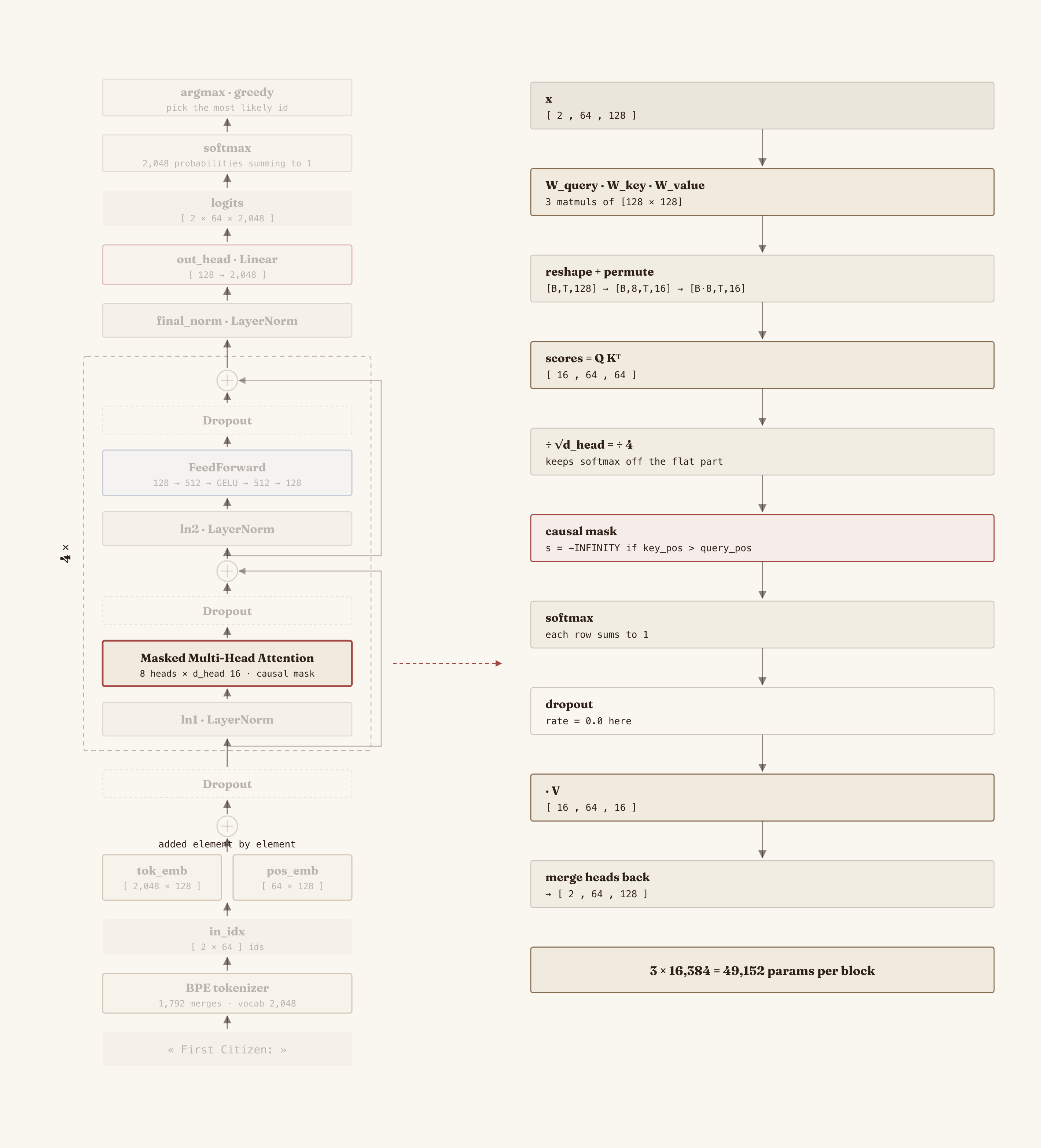
We already have the central mechanism complete, and we already have something that really uses context. What's left is building the model around it. Stacking this several times, making it trainable, and giving it an output that returns tokens.

The model

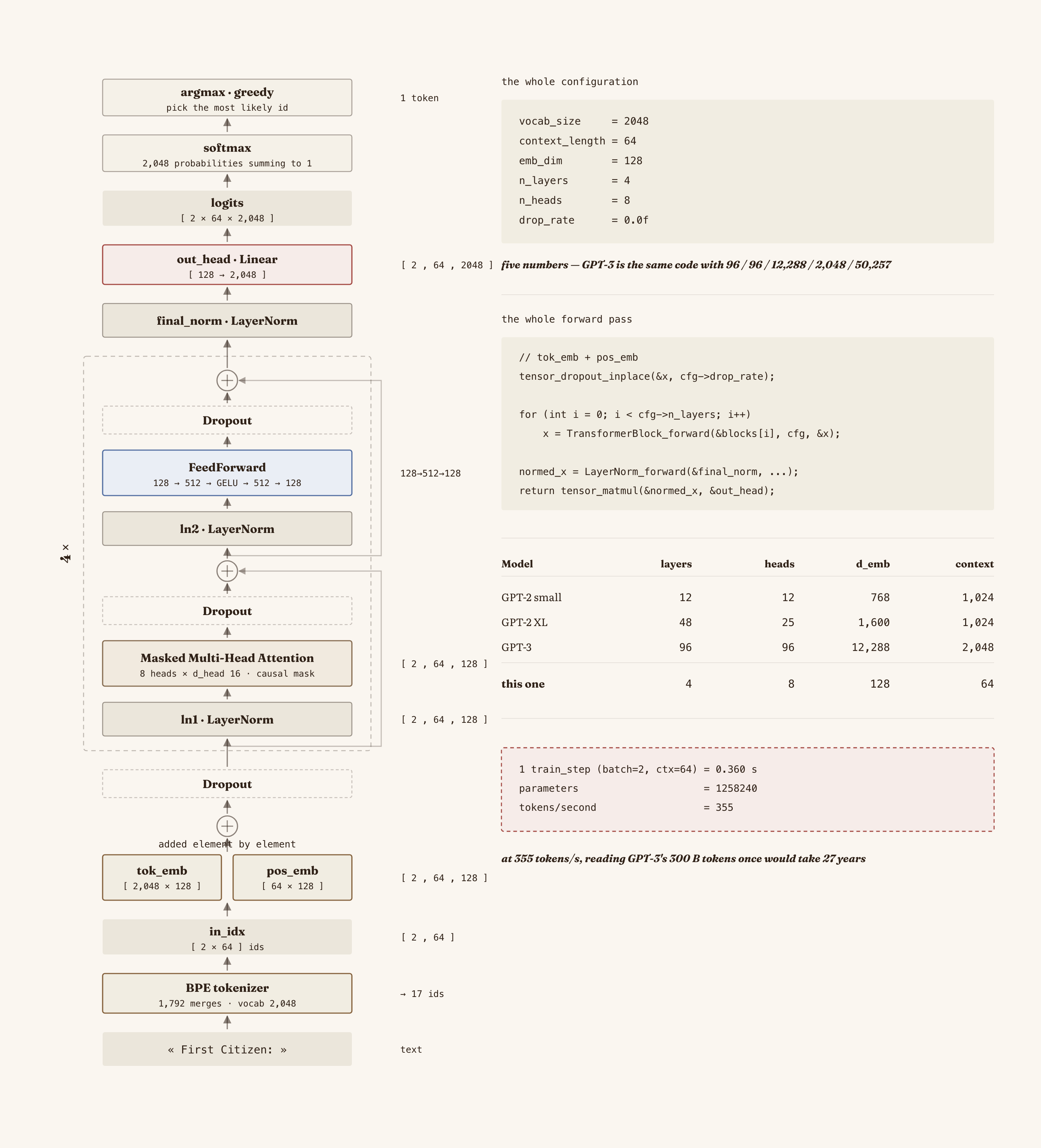
The complete model architecture, from the embeddings to the output head — The complete machine, with the shape of the tensor at each step.

We already have the text turned into vectors and the mechanism that lets them look at each other. What's left is the complete machine and connecting what we already built.

They all exist because without them training doesn't work.

Why this doesn't train on a laptop

I timed a single training step of our model on a MacBook Air M2 with 8gb of RAM:

=== speed ===
  1 train_step (batch=2, ctx=64) = 0.360 s
  params counted = 1258240
  tokens per step = 128
  tokens/second = 355

355 tokens per second. With that, let's see what would happen if I wanted to train GPT-3 here.

GPT-3 was trained on 300 billion tokens. At 355 tokens per second, our 1.26 million parameter model would take 27 years just to read that amount of text once.

But GPT-3 doesn't have 1.26 million parameters, it has 175 billion. That's 139,000 times more, and the work per token grows more or less just as fast. Multiplying:

27 \text{ years} \times 139{,}000 \approx 3.7 \text{ million years}

And that's assuming the memory was enough. In 32 bit float:

	GPT-3	ours
Weights	700 GB	5 MB
Gradients	700 GB	5 MB
AdamW states ( $m$ and $v$ )	1,400 GB	10 MB
Total to train	2.8 TB	20 MB

My laptop has 8 GB. I'd need 350 times more RAM, before doing a single multiplication.

That's why this project is a 1.26 million parameter model and not a 175 billion one. It's a limitation of electricity and of money :). The architecture I'm going to build is the same. The only difference is the five numbers in the configuration. I'll explain it below.

LayerNorm

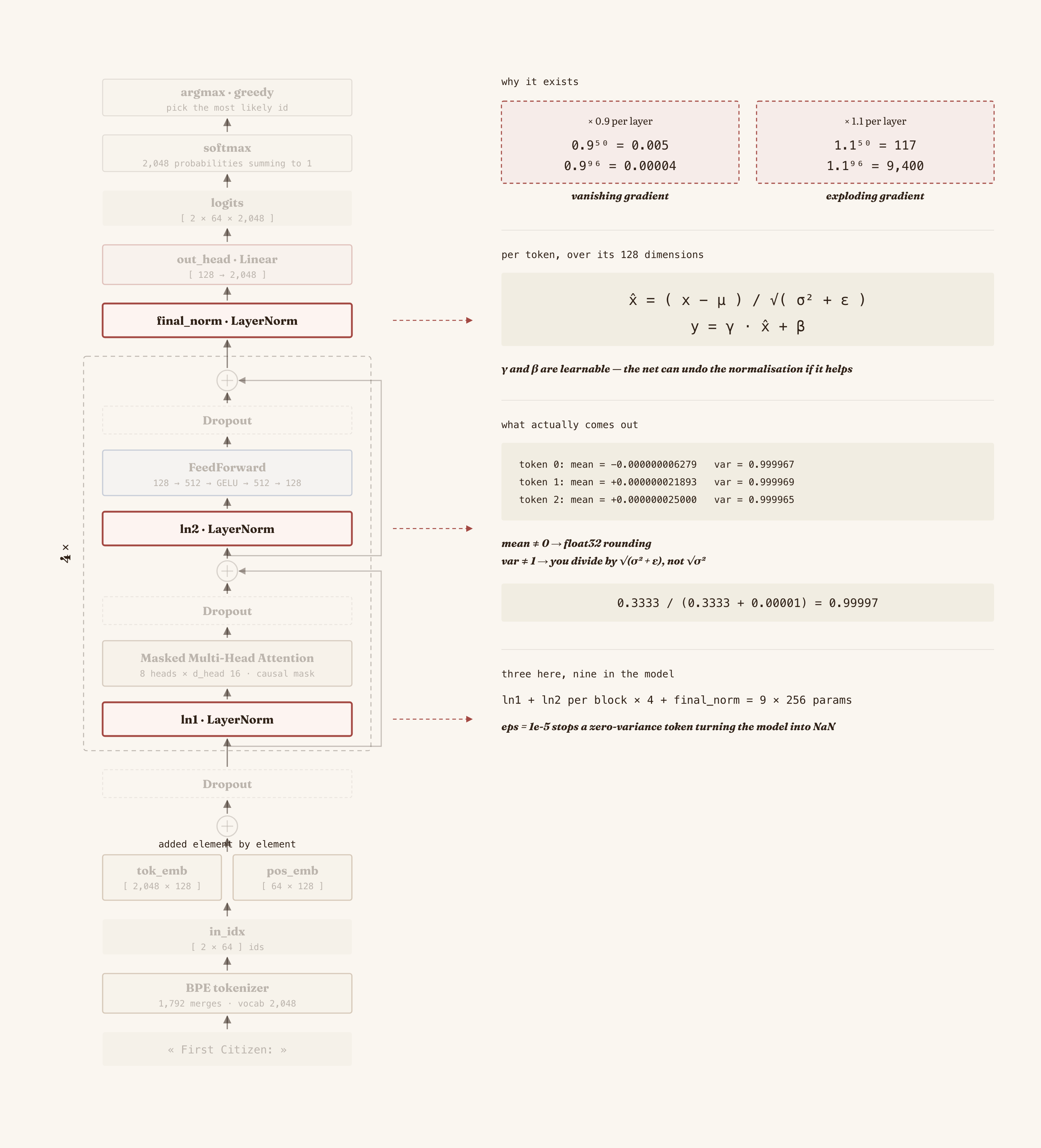
Gradients that vanish or explode

When you train a network, the error propagates from the last layer toward the first multiplying derivatives, layer by layer (that's the chain rule).

If each layer multiplies by something slightly less than 1, let's say $0.9$ :

0.9^{50} = 0.005 \qquad 0.9^{96} = 0.00004

The gradient reaches the first layers turned into a very small number. Those layers stop learning, not because they're fine, but because they receive no signal. That's the vanishing gradient.

And if each layer multiplies by something slightly greater than 1, let's say $1.1$ :

1.1^{50} = 117 \qquad 1.1^{96} = 9{,}400

The gradient arrives gigantic, the optimizer takes a big jump, and the weights go to NaN. That's the exploding gradient.

To solve it you can't let the magnitudes run away. Keep them in a fixed range, layer by layer, by force.

That's normalizing.

The formula

For each token, separately, its 128 numbers are taken and rescaled so they have mean 0 and variance 1:

\hat{x}_d = \frac{x_d - \mu}{\sqrt{\sigma^2 + \epsilon}}

Where $\mu$ and $\sigma^2$ are the mean and the variance of that token only, computed over its 128 dimensions.

float mean = tensor_mean(&token_vec);
float var  = tensor_var(&token_vec);
float r = 1.0f / sqrtf(var + self->eps);

for (int d = 0; d < x->shape[2]; d++) {
    float xhat = (token_vec.data[d] - mean) * r;
    tensor_set(&normed_x, coords,
               (self->scale.data[d] * xhat) + self->shift.data[d]);
}

The mean doesn't land on zero

Running it:

=== LayerNorm, real mean and variance ===
  token 0: mean = -0.000000006279   var = 0.999967312228
  token 1: mean = +0.000000021893   var = 0.999969047551
  token 2: mean = +0.000000025000   var = 0.999965022369

The mean isn't 0, it's $-6.3 \times 10^{-9}$ . And the variance isn't 1, it's $0.99997$ .

The one about the mean is floating point precision. A 32 bit float has about 7 decimal digits of precision. When you add 128 numbers and divide, each operation rounds a little, and the roundings don't cancel out perfectly. You subtract the mean from each element, but the mean you're subtracting already came with error, so the mean of the result lands on the order of $10^{-8}$ instead of exactly 0. In mathematics it's zero. On a computer, it's different.

The one about the variance... look at the formula... you divide by $\sqrt{\sigma^2 + \epsilon}$ , not by $\sqrt{\sigma^2}$ . That $\epsilon$ you add makes you divide by a slightly bigger number than you should, so the resulting variance lands slightly below 1:

\frac{\sigma^2}{\sigma^2 + \epsilon} = \frac{0.3333}{0.3333 + 0.00001} = 0.99997

What the `eps` is for

self->eps = 1e-5; // prevents division by zero

It's there for the case where a token has zero variance, that is, its 128 numbers are all identical. Without the eps you'd be dividing by zero and you get inf, and then inf - inf = NaN, and the NaN eats the entire model in the next matmul.

Which means the eps is insurance that costs an error of $3 \times 10^{-5}$ in the variance and saves you from training dying.

Another detail is that I compute the variance dividing by $n$ , not by $n-1$ .

float tensor_var(Tensor *t) {
    float sum = 0.0f;
    float mean = tensor_mean(t);
    for (int i = 0; i < t->size; i++) {
        sum += powf(t->data[i] - mean, 2);
    }
    return sum / t->size;
}

Dividing by $n-1$ (Bessel's correction) is the right thing when you have a sample and want to estimate the variance of a bigger population you didn't see. But we have the complete 128 dimensions, not a sample of them. We're not estimating anything, we're describing what we have. So you divide by $n$ . In PyTorch this is the unbiased=False that shows up in tutorials with no explanation.

After all the work of forcing mean 0 and variance 1, there are two parameters that move it again:

self->scale = tensor_create_ones(scale_and_shift_shape, 1);
self->shift = tensor_create_zeros(scale_and_shift_shape, 1);

y_d = \gamma_d \cdot \hat{x}_d + \beta_d

Multiply by scale and add shift, with a different value for each of the 128 dimensions, and both trainable.

The three positions

In the model there are exactly three LayerNorms:

ln1, before attention.
ln2, before the feed-forward network.
final_norm, at the very end, before converting to tokens.

The first two repeat in each block (4 blocks × 2 = 8 instances), the third is unique.

GELU and the feed-forward network

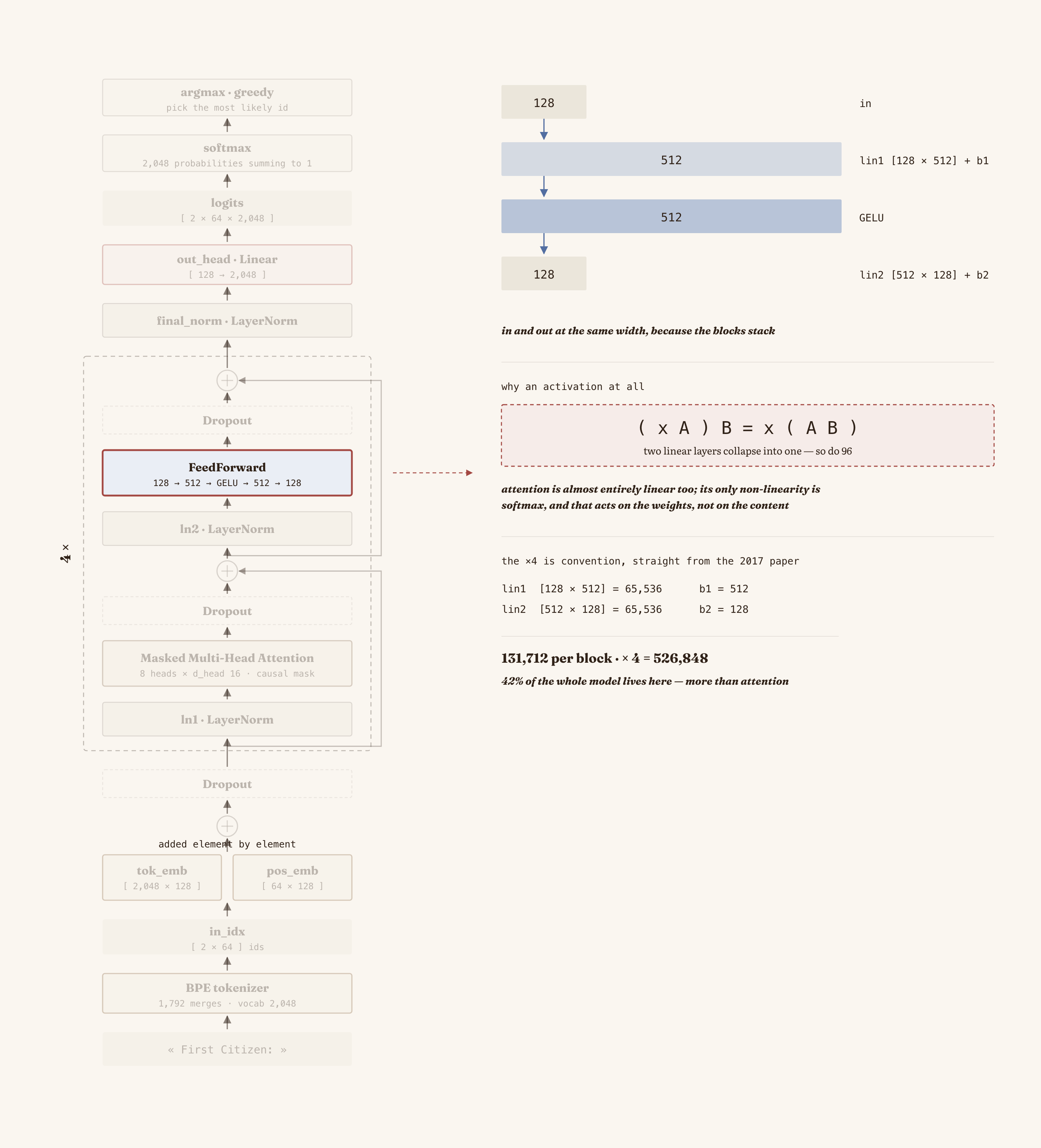
Close-up of the feed-forward network with GELU inside the architecture — 128 → 512 → GELU → 128. 42% of the parameters live here.

What is an activation function for?. If your layer is a matrix multiplication, stacking two layers is:

(x A) B = x (AB)

The product $AB$ is another matrix. So two linear layers are mathematically identical to a single linear layer with the matrix $AB$ . 4 layers are one, and 96 layers are one.

Without activation functions, all the work of stacking blocks wouldn't work... you could precompute the product of all the matrices and have exactly the same model in a single operation.

The only thing that breaks that collapsibility is putting something non linear between layer and layer. That's an activation function. It's not there to imitate biological neurons or anything like that, it's there because without it the network can't represent more than a straight line, no matter how deep you make it. Normally activation functions are only included when the neural network is very deep.

And this also explains why attention alone isn't enough. Attention is almost entirely linear... projections, dot products, weighted sums. Its only non linearity is the softmax, and it acts on the weights, not on the content.

ReLU vs GELU

The simplest activation is ReLU. If it's negative, zero; if it's positive, leave it as is. Our model uses GELU, which does almost the same thing but smooth.

=== GELU vs ReLU ===
     x        ReLU(x)      GELU(x)
   -3.0      +0.000      -0.00364
   -2.0      +0.000      -0.04540
   -1.0      +0.000      -0.15881
   -0.5      +0.000      -0.15429
   -0.1      +0.000      -0.04602
   +0.0      +0.000      +0.00000
   +0.1      +0.100      +0.05398
   +0.5      +0.500      +0.34571
   +1.0      +1.000      +0.84119
   +2.0      +2.000      +1.95460
   +3.0      +3.000      +2.99636

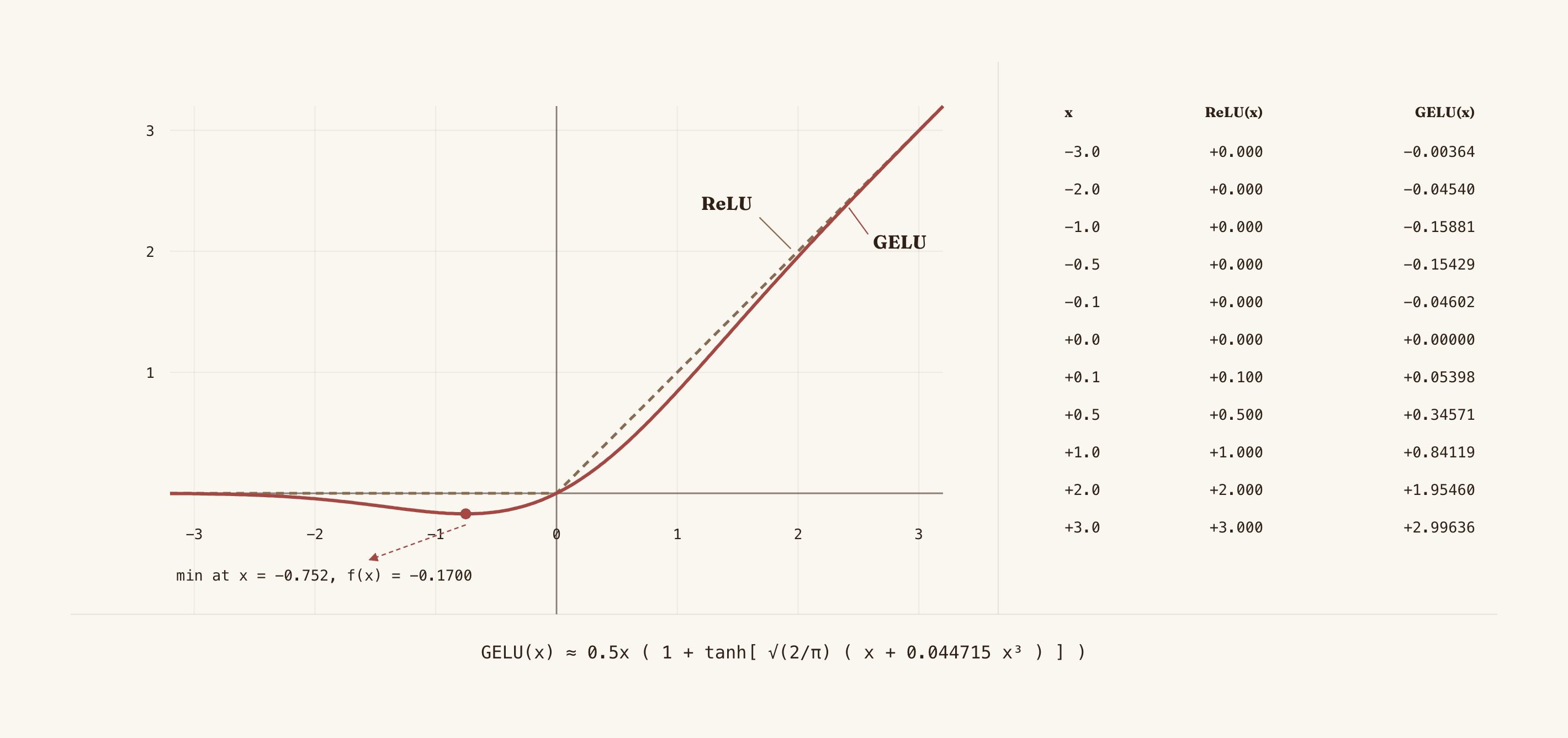
ReLU with its elbow against GELU with its smooth curve and its minimum in the negatives — ReLU's elbow against GELU's curve, with its minimum in the negatives.

The real GELU is defined with the cumulative distribution function of the normal, $\text{GELU}(x) = x \cdot \Phi(x)$ , which reads as "let $x$ through in proportion to the probability that a standard normal is less than $x$ ". The problem is that $\Phi$ is computed with the error function. So an approximation with hyperbolic tangent is used:

\text{GELU}(x) \approx 0.5x\left(1 + \tanh\left[\sqrt{\tfrac{2}{\pi}}\left(x + 0.044715x^3\right)\right]\right)

void GELU(Tensor *x) {
    // Hyperbolic Tangent (Tanh) Approximation
    for (int i = 0; i < x->size; i++) {
        // Approximate Cumulative Distribution Function (CDF)
        float cdf = 1 + tanhf(sqrtf(2 / M_PI) * (x->data[i] + (0.044715 * powf(x->data[i], 3))));
        x->data[i] = 0.5 * x->data[i] * cdf;
    }
}

The feed-forward network

With GELU we can now build the second half of the block.

void FeedForward_init(FeedForward *self, GPT_CONFIG *cfg) {
    const int lin1_shape[2] = {cfg->emb_dim, 4 * cfg->emb_dim};   // 128 -> 512
    self->lin1 = tensor_create_random(lin1_shape, 2, 0.02);
    self->b1 = tensor_create_zeros((int[]){4 * cfg->emb_dim}, 1);

    const int lin2_shape[2] = {cfg->emb_dim * 4, cfg->emb_dim};   // 512 -> 128
    self->lin2 = tensor_create_random(lin2_shape, 2, 0.02);
    self->b2 = tensor_create_zeros((int[]){cfg->emb_dim}, 1);
}

128 \longrightarrow 512 \longrightarrow \text{GELU} \longrightarrow 128

The non linearity can only separate things that are separable in the space where it lives. If you stay in 128 dimensions, GELU has little room. By projecting to 512 you give the model a wider space where the things that were mixed up can settle into different regions, there you apply the non linearity, and then you come back. The factor of 4 is convention (it comes from the 2017 paper and everyone copied it).

It goes in and comes out at the same dimension because the blocks get stacked.

The transformer block

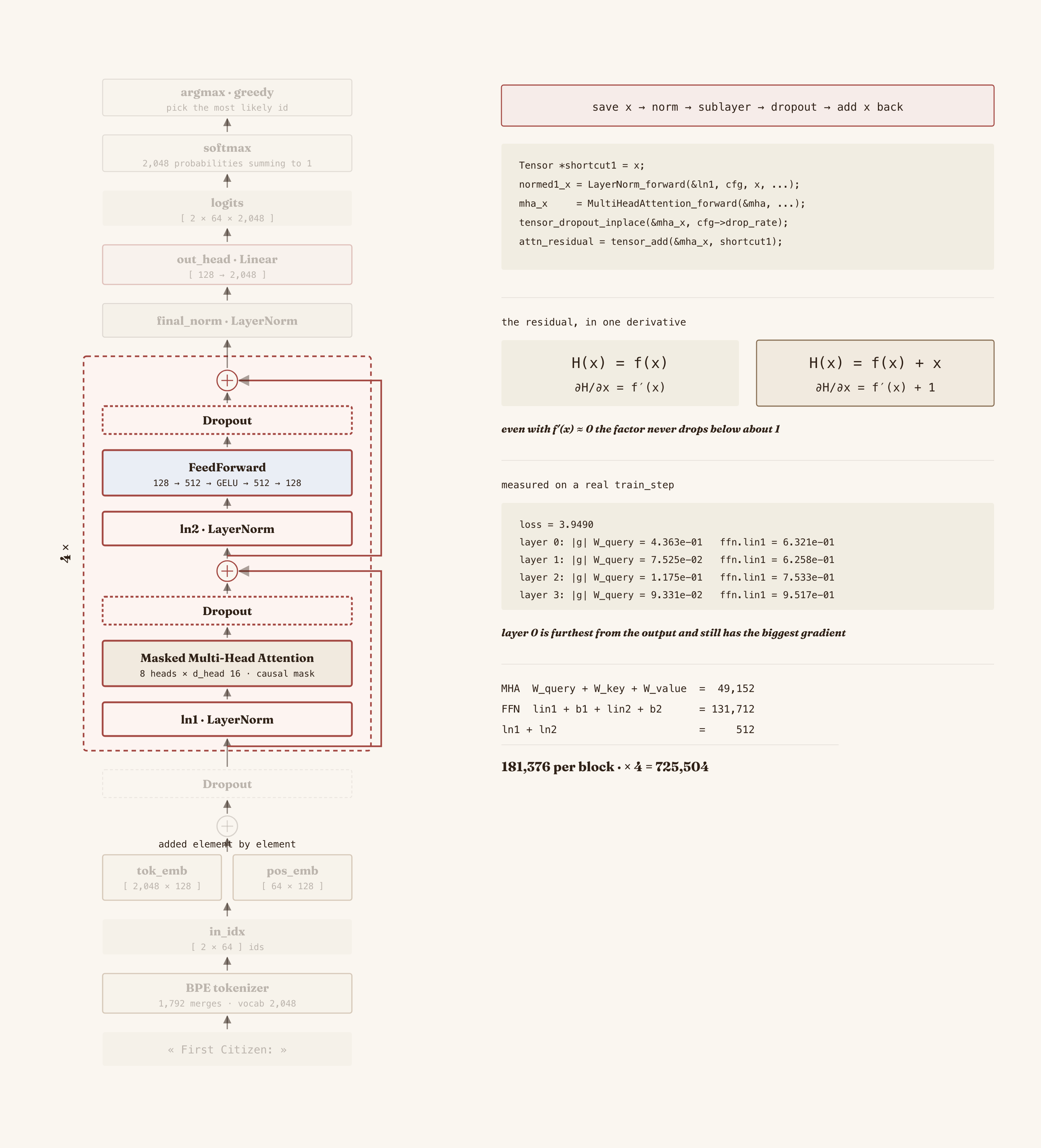
Close-up of the complete transformer block inside the architecture — The block that repeats 4 times here and 96 times in GPT-3.

Now we put the four pieces together.

The residual connections

LayerNorm doesn't fix the vanishing gradient problem. LayerNorm controls the scale of the activations, but the gradient still has to cross all the layers multiplying itself, and it can still die on the way. Normalizing doesn't change the fact that you're multiplying 96 numbers.

The solution is a single sum. Instead of the layer returning its result:

H(x) = f(x)

you add its own input to it:

H(x) = f(x) + x

And that's it. That's a residual connection, a shortcut.

Why it works: take the derivative of both versions.

\frac{\partial H}{\partial x} = f'(x) \qquad \text{vs} \qquad \frac{\partial H}{\partial x} = f'(x) + 1

That $+1$ is everything. When the gradient passes backward through this layer, it gets multiplied by $f'(x) + 1$ instead of by $f'(x)$ . And even if $f'(x)$ is $0.0001$ , even if the layer is completely dead, the factor never drops below approximately 1. The gradient can't vanish, because there's a path where it passes through multiplying by one.

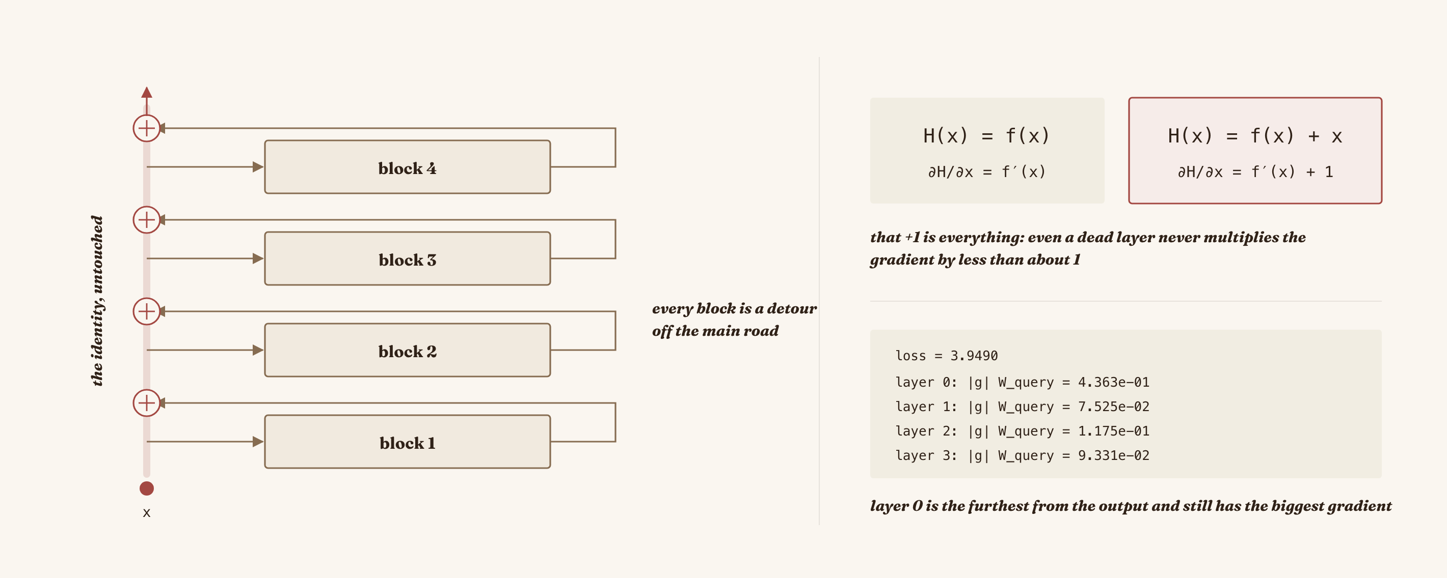
The residual connection as a highway that crosses all the blocks without transforming — The highway that crosses the blocks without transforming: the +1 of the gradient.

And this can be measured. I ran a real train_step and printed the norm of the gradient that reached each layer:

=== gradient norm per layer (a real train_step) ===
  loss = 3.9490
  layer 0: |g| W_query = 4.363e-01   |g| ffn.lin1 = 6.321e-01
  layer 1: |g| W_query = 7.525e-02   |g| ffn.lin1 = 6.258e-01
  layer 2: |g| W_query = 1.175e-01   |g| ffn.lin1 = 7.533e-01
  layer 3: |g| W_query = 9.331e-02   |g| ffn.lin1 = 9.517e-01
  tok_emb: |g| = 1.879e+00   out_head: |g| = 1.728e+00

Layer 0 is the farthest from the output. And its gradient in W_query is $0.436$ , which is the biggest of the four layers, five times bigger than layer 1's. In the FFN all four are in the same order of magnitude, between $0.63$ and $0.95$ . The signal arrived complete.

Being honest, with 4 layers this is a soft test. Vanishing is a problem of deep networks, and 4 isn't deep, so it would probably survive even if I took the shortcuts away.

The order

Tensor TransformerBlock_forward(TransformerBlock *self, GPT_CONFIG *cfg, Tensor *x) {
    Tensor *shortcut1 = x;
    Tensor normed1_x = LayerNorm_forward(&self->ln1, cfg, x, NULL, NULL);
    Tensor mha_x = MultiHeadAttention_forward(&self->mha, cfg, &normed1_x);
    tensor_dropout_inplace(&mha_x, cfg->drop_rate);
    Tensor attn_residual = tensor_add(&mha_x, shortcut1);

    Tensor *shortcut2 = &attn_residual;
    Tensor normed2_x = LayerNorm_forward(&self->ln2, cfg, &attn_residual, NULL, NULL);
    Tensor ffn_x = FeedForward_forward(&self->ffn, &normed2_x);
    tensor_dropout_inplace(&ffn_x, cfg->drop_rate);
    Tensor block_out = tensor_add(&ffn_x, shortcut2);

    return block_out;
}

That's the transformer block, the unit that repeats 4 times in our model and 96 times in GPT-3.

The pattern is the same twice:

save x  ->  normalize  ->  submodule  ->  dropout  ->  add the saved x

The complete model

With the block ready, the whole model is putting everything together:

typedef struct {
    Tensor tok_emb;                 // [vocab, emb]
    Tensor pos_emb;                 // [ctx, emb]
    TransformerBlock *trf_blocks;   // n_layers blocks
    LayerNorm final_norm;
    Tensor out_head;                // [emb, vocab]
} GPTModel;

And the forward pass:

Tensor GPTModel_forward(GPTModel *self, GPT_CONFIG *cfg, Tensor in_idx) {
    // ... tok_emb + pos_emb (the block from chapter 2) ...
    tensor_dropout_inplace(&x, cfg->drop_rate);

    for (int i = 0; i < cfg->n_layers; i++) {
        Tensor next_block = TransformerBlock_forward(&self->trf_blocks[i], cfg, &x);
        tensor_free(&x);
        x = next_block;
    }

    Tensor normed_x = LayerNorm_forward(&self->final_norm, cfg, &x, NULL, NULL);
    tensor_free(&x);

    Tensor logits = tensor_matmul(&normed_x, &self->out_head);
    tensor_free(&normed_x);

    return logits;
}

That's an LLM. Embeddings, a for with 4 iterations, a normalization, and a final multiplication. If it seems like little to you, it's because it is little. The entire GPT architecture fits in this function. What doesn't fit in any function are the 1.26 million numbers.

out_head is $[128, 2048]$ , so it converts each token's 128 dimensional vector into 2,048 numbers, one for each token in the vocabulary. Those numbers are called logits, and they're the raw scores of "how likely is it that the next token is this one". We started by turning text into vectors and we end up turning vectors into a score for every possible piece of text.

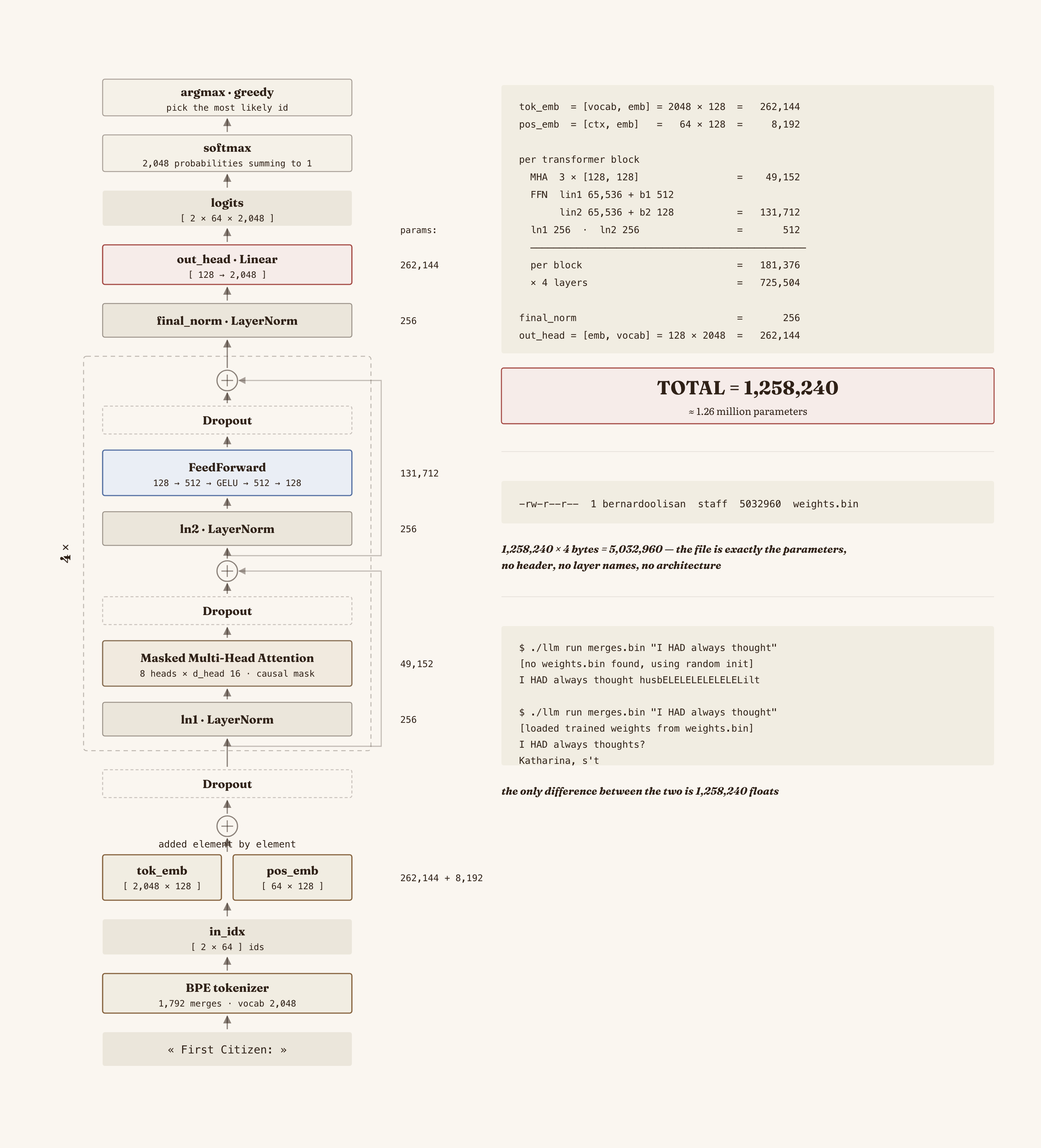
Counting the parameters

Embeddings:
- tok_emb = [vocab, emb] = 2048 × 128 = 262,144
- pos_emb = [ctx, emb]   = 64 × 128   = 8,192

One transformer block:
- MHA: W_query, W_key, W_value, each [128, 128] = 16,384 → 3 × 16,384 = 49,152
- FFN: lin1 [128, 512] = 65,536 | b1 = 512 | lin2 [512, 128] = 65,536 | b2 = 128
       subtotal = 131,712
- ln1: scale + shift = 256      | ln2: scale + shift = 256
- Total per block = 181,376

× 4 layers = 725,504

final_norm = 256
out_head = [emb, vocab] = 128 × 2048 = 262,144

TOTAL = 1,258,240  ≈ 1.26M parameters

Saving the parameters

When training finishes, this is what's left on disk:

-rw-r--r--  1 bernardoolisan  staff  5032960  weights.bin

If we compute: $1{,}258{,}240 \times 4 = 5{,}032{,}960$ .

The file is exactly the parameters times 4 bytes. There's no header, no metadata, no layer names, no description of the architecture. It's a strip of floats glued together:

void save_weights(const char *path, ParamList *pl) {
    FILE *f = fopen(path, "wb");
    for (int i = 0; i < pl->count; i++)
        fwrite(pl->params[i]->data, sizeof(float), pl->params[i]->size, f);
    fclose(f);
}

When someone "releases a model", they release a file of numbers and a description of the shape. The only difference is that their file weighs 700 GB and mine 5 MB.

Generating text

Now, we have to use it.

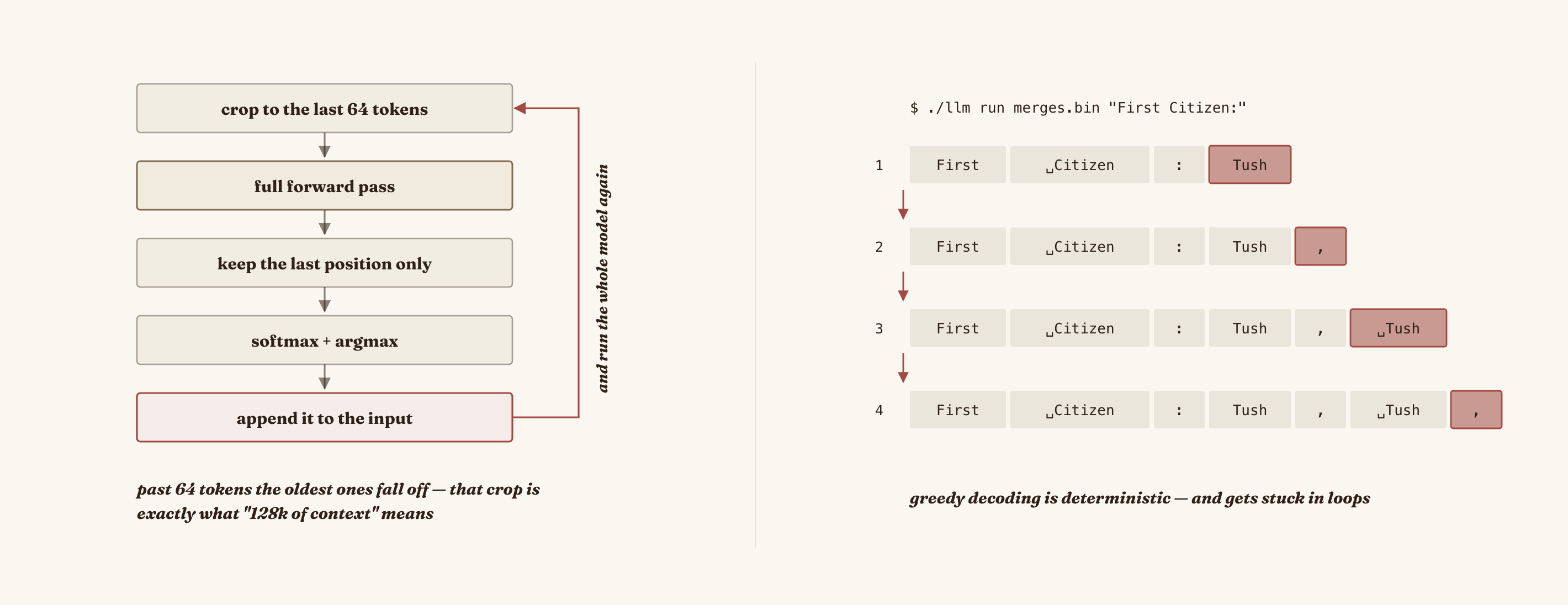
The model produces 2,048 logits for each position. To generate text, we only care about the last position, because it's the one that predicts what comes after everything we gave it. A token is picked, glued to the end of the input, and the whole model is run again. That's called autoregressive generation. The output becomes part of the input.

Autoregressive generation: each produced token becomes part of the input — The output becomes input, one token at a time.

Tensor generate_text(GPTModel *model, GPT_CONFIG *cfg, Tensor idx, int max_new_tokens) {
    for (int i = 0; i < max_new_tokens; i++) {
        // 1. trim to the last context_length tokens
        const int bound = MIN(idx.shape[1], cfg->context_length);
        // ... copy the last `bound` tokens into idx_cond ...

        // 2. full forward pass
        Tensor logits = GPTModel_forward(model, cfg, idx_cond);

        // 3. keep only the last position
        for (int d = 0; d < logits.shape[2]; d++) {
            const int coords[3] = {0, logits.shape[1] - 1, d};
            last_logit_vec[d] = tensor_get(&logits, coords, 3);
        }
        softmax(last_logit_vec, logits.shape[2]);

        // 4. pick the most likely one (greedy)
        int token_id = 0;
        for (int d = 0; d < logits.shape[2]; d++) {
            if (last_logit_vec[d] > last_logit_vec[token_id]) token_id = d;
        }

        // 5. glue it to the end and repeat
        Tensor new_idx = tensor_cat(&idx, &idx_next, 1);
        idx = new_idx;
    }
    return idx;
}

When the text goes past 64 tokens, the oldest ones simply fall off. They get trimmed and the model never knew they existed. When you hear that a model "has 128k of context", that's literally the size of this trim. Everything that falls outside, falls outside.

Always picking the maximum is called greedy decoding, and it's deterministic. The same input text produces exactly the same output every time. There's no creativity or randomness. And that's also why it gets stuck in loops, if the most likely token after "Tush, " is "Tush", it keeps repeating Tush, Tush, Tush forever, because it has no mechanism to prefer anything else.

This is the trained model:

$ ./llm run merges.bin "First Citizen:"
[loaded trained weights from weights.bin]
First Citizen: wrong you wrong, you do you w

$ ./llm run merges.bin "ROMEO:"
ROMEO: musice, I
you see him

$ ./llm run merges.bin "I HAD always thought"
I HAD always thoughts?
Katharina, s't

That's 1.26 million parameters. It learned the shape of language, spelling, formatting, syntax. What it doesn't have is coherence beyond a few words, and that's exactly what I expected, because its context window is 64 tokens and its capacity is four layers.

The distance between this and ChatGPT is numbers. It's the same code with 139,000 times more parameters, and 300 billion tokens instead of one book.

The complete GPT architecture: embeddings, N transformer blocks, final norm and output head — The 1,258,240 parameters, and where each one lives.

Training

The model throws out 2,048 logits per position. If we pass them through softmax, we have a probability for each token in the vocabulary. "I think the next one is " the " with 3%, "y " with 0.4%...".

And we know the right answer, because the targets we saw earlier are the text shifted one place. So, to score the model we only have to ask, how much probability did you give to the token that actually came next?

If it gave it 0.9, it's doing well. If it gave it 0.0001, it's doing badly. And out of that comes the loss function, which is only 3 steps:

L = -\frac{1}{N}\sum_{i=1}^{N} \log p_i

Where $p_i$ is the probability the model assigned to the correct token at position $i$ .

The logarithm. Without it you'd have to multiply the probabilities of all the positions, and multiplying thousands of numbers smaller than 1 gives you something so tiny that a float rounds it to zero. The logarithm turns products into sums... $\log(ab) = \log a + \log b$ . Adding is stable, multiplying isn't.

The negative sign. The logarithm of a number between 0 and 1 is always negative. If the model gave 0.9 to the correct token, $\log(0.9) = -0.105$ ; if it gave 0.0001, $\log(0.0001) = -9.2$ . Flipping the sign turns that into a scale where bigger is worse, which is what you want if you're going to minimize.

The average. So the number doesn't depend on how many tokens you put in the batch. That way a loss of 3.9 means the same thing with a batch of 2 as with a batch of 2,000.

In C, it looks like this:

softmax(logit_vec, logits->shape[2]);
int target_token_id = (int)tensor_get(targets, coords, 2);
target_probabilities[(b * logits->shape[1]) + pos] = logit_vec[target_token_id];
// ...
log_probabilities[p] = logf(target_probabilities[p]);
float average_log_prob = mean(log_probabilities, ...);
float loss = average_log_prob * -1;

This is called cross entropy loss. In PyTorch, F.cross_entropy(logits, targets), and it's exactly what's above. It's called that because it measures the "distance" between two probability distributions... the model's and the real one.

Model quality

With those two numbers we can already prove it. An untrained model should be choosing uniformly among the 2,048 tokens, that is, giving each one a probability of $\frac{1}{2048}$ . If that's true, its loss has to be exactly:

L = -\log\left(\frac{1}{2048}\right) = \log(2048) = 7.6246

That's the number the theory predicts. I ran the model with random weights and with the trained weights, over the same batch:

=== loss: untrained vs trained (same batch) ===
  vocab_size = 2048
  theoretical loss of a model guessing at random = ln(2048) = 7.6246
  loss with random weights   = 7.6226   (perplexity 2043.8)
  loss with trained weights  = 3.9490   (perplexity 51.9)

7.6226 measured against 7.6246 predicted. They match to three decimals, and the perplexity came out at 2043.8 out of a maximum of 2048.

The loss is confirming that the untrained model spreads its confidence almost perfectly evenly across the 2,048 options. It has no preference for anything. The whole machine we built (the embeddings, the 32 attention heads, the four FFNs, the nine LayerNorms) is working, and its behavior is indistinguishable from rolling a 2,048 sided die.

And trained, the same machine drops to perplexity 51.9. It went from choosing among 2,048 options to choosing among 52.

This is how the difference looks in text:

$ ./llm run merges.bin "I HAD always thought"
[no weights.bin found, using random init]
I HAD always thought husbELELELELELELELilt

$ ./llm run merges.bin "I HAD always thought"
[loaded trained weights from weights.bin]
I HAD always thoughts?
Katharina, s't

The only difference between husbELELELELELELELilt and Katharina are the 1,258,240 floats of weights.bin.

And well, that's all. I wanted to explain the training machine I built in C, but the truth is it would be double what I wrote in this article, and the idea of this article is to explain how an LLM works from scratch. This has been a very big challenge for me because implementing something like this in C is always complicated. The truth is that people should understand how the things they use work, there are far too many who talk about artificial intelligence without knowing what it is, or how it works, and the worst part is that they reach conclusions that contaminate other people.

If you want to see how all the code looks, I'm leaving it here: https://github.com/BernardoOlisan/llm

Thanks :)